Ch 3 — OS, Docker, and Kubernetes Tuning for GPU-Based Environments
Even with highly optimized GPU code and libraries, system-level bottlenecks can limit performance in large-scale AI training. The fastest GPU is only as good as the environment feeding it data and instructions. In this chapter, we explore how to tune the operating system and container runtime to let GPUs reach their full potential. We begin by exploring the foundational GPU software stack. We then dive into key CPU and memory optimizations such as NUMA affinity and hugepages. These ensure that data flows efficiently from storage through the CPU to the GPU. In parallel, we discuss critical GPU driver settings like persistence mode, Multi-Process Service (MPS), and Multi-Instance GPU (MIG) partitions. These help maintain maximum GPU uti‐ lization by reducing overhead and synchronizing resources effectively. Using solutions like the NVIDIA Container Toolkit, Container Runtime, Kubernetes Topology Manager, and Kubernetes GPU Operator, you can create a unified and highly optimized software stack for GPU environments. These solutions enable effi‐ cient resource allocation and workload scheduling across single-node and multinode GPU environments—and ensure GPU capabilities are fully utilized. Along the way, you’ll build intuition for why these optimizations matter. In essence, they minimize latency, maximize throughput, and ensure your GPUs are constantly fed with data and operating at their peak performance. The result is a robust, scalable system that delivers significant performance gains—and a high goodput percentage— for both training and inference workloads.
Operating System The operating system (OS) is the foundation that everything runs on. GPU servers typically run a Linux distribution such as Ubuntu Server LTS or Red Hat with an updated kernel that supports the latest GPU hardware. The NVIDIA driver installs kernel modules that create device files like /dev/nvidia0, /dev/nvidia1, and /dev/ nvidia2—one for each GPU. The driver also creates /dev/nvidiactl for driver con‐ trol operations, /dev/nvidia-uvm for unified virtual memory, and /dev/nvidiamodeset for mode-setting and buffer management. The OS manages CPU scheduling, memory, networking, and storage—all of which should be tuned for high GPU throughput. As such, the OS should be configured to avoid interfering with GPU tasks. For example, GPU nodes should disable swapping or set vm.swappiness to 0 to avoid any OS-initiated memory swapping that could interfere with GPU workloads. Part of our job as performance engineers is to adjust these OS settings to set the GPUs up for maximum performance. A GPU-focused server might want to run additional daemons, or background pro‐ cesses, such as the NVIDIA Persistence Daemon to keep the GPU driver and hard‐ ware context loaded and ready—even when no GPU jobs are running. In addition, the Fabric Manager manages GPU interconnect topology. And the NVIDIA Data Center GPU Manager (DCGM) monitors GPU system health metrics.
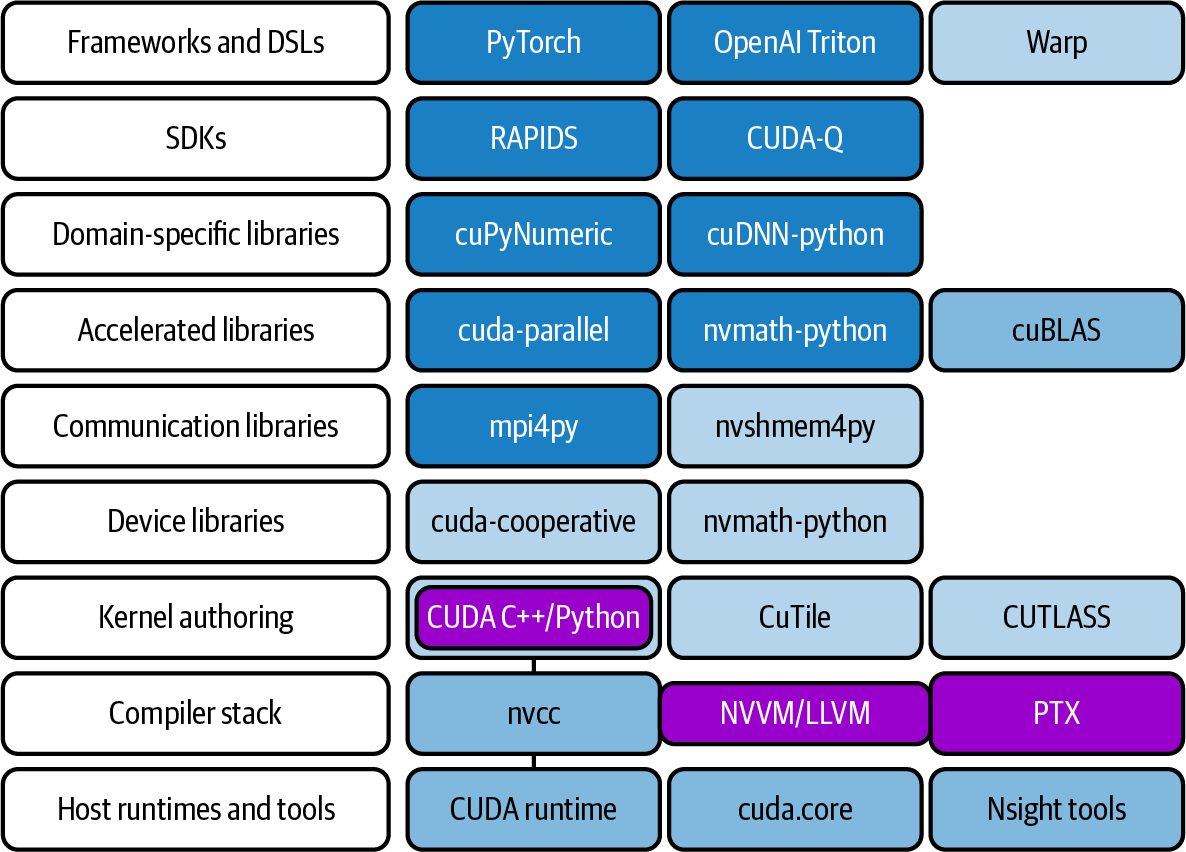
NVIDIA Software Stack Running a multi-petaFLOP GPU cluster involves more than just writing high-level PyTorch, TensorFlow, or JAX code. There is a whole software stack underpinning GPU operations, and each layer can affect performance. Figure 3-1 shows a common set of frameworks, libraries, compilers, runtimes, and tools used to develop and pro‐ ductionize modern LLM workloads, including PyTorch, cuDNN, cuBLAS, CUT‐ LASS, CUDA C++, nvcc, and the CUDA Runtime API (e.g., CUDA tools, driver, etc.). In addition, the NVIDIA GPU and CUDA ecosystem embraces Python libraries and allows you to create CUDA kernels in Python using frameworks like OpenAI’s Triton domain-specific language (DSL) and NVIDIA’s Warp framework—as well as NVIDIA’s CUDA Python, cuTile, and CUTLASS libraries.
56 | Chapter 3: OS, Docker, and Kubernetes Tuning for GPU-Based Environments
Figure 3-1. Common set of frameworks, libraries, compilers, runtimes, and tools used to develop and productionize modern LLM workloads
GPU Driver At the base is the NVIDIA GPU driver, which interfaces between the Linux OS and the GPU hardware. The driver manages low-level GPU operations, including mem‐ ory allocation on the device, task scheduling on GPU cores, and partitioning the GPU for multitenant usage. The GPU driver turns on the GPUs’ features and keeps the hardware fed with work. It’s important to keep the NVIDIA driver up-to-date. New driver releases often unlock performance improvements and support the latest GPU architectures and CUDA features. Tools such as nvidia-smi come with the driver and allow you to monitor tempera‐ tures, measure utilization, query error-correcting code (ECC) memory status, and enable different GPU modes like persistence mode.
CUDA Toolkit and Runtime On top of the driver sits the CUDA Runtime and libraries called the CUDA Toolkit. The toolkit includes the CUDA compiler, nvcc, used to compile CUDA C++ kernels. When compiled, CUDA programs link against the CUDA runtime (cudart). The CUDA runtime communicates directly with the NVIDIA driver to launch work and allocate memory on the GPU.
NVIDIA Software Stack | 57
Additionally, the CUDA Toolkit provides many optimized libraries: cuDNN for neu‐ ral network primitives, cuBLAS for linear algebra, NCCL for multi-GPU communica‐ tion, etc. As such, it’s critical to use the latest CUDA Toolkit version that supports your GPU’s compute capability (CC) since an up-to-date toolkit has the latest com‐ piler optimizations and libraries specific to your GPU. We will cover the CUDA com‐ piler and programming model—as well as CUDA (and PyTorch) optimizations—in more detail in the upcoming chapters.
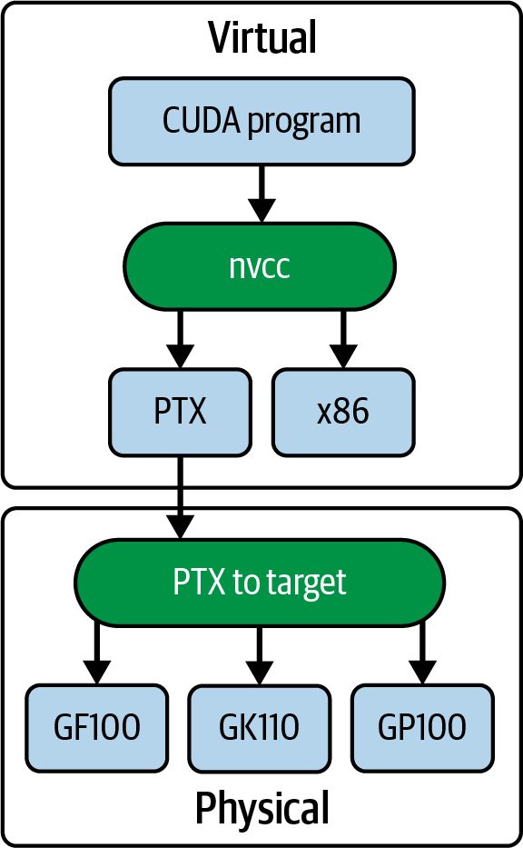
CUDA Forward and Backward Compatibility Across GPU Hardware Generations An important feature of NVIDIA’s GPU programming model is its compatibility across hardware generations. When you compile CUDA code, the resulting binary includes virtual, or intermediate, PTX code as well as physical device code (e.g., ARM, x86, GPU instructions), as shown in Figure 3-2.
Figure 3-2. Using nvcc to compile a CUDA program into PTX—and ultimately the lowlevel instructions for the GPU target device
This allows newer GPUs to just-in-time (JIT) compile the PTX so your program runs on future architectures—and allows newer GPUs to execute older binary code for prior architectures. This compatibility is achieved through NVIDIA’s fatbinary model, which contains PTX for future-proofing and CUBIN, or architecture-specific CUDA device code binaries, for known architectures.
58 | Chapter 3: OS, Docker, and Kubernetes Tuning for GPU-Based Environments
CUBIN is the binary produced by nvcc using the -cubin option. It contains compiled GPU streaming assembler (SASS) instructions for a given NVIDIA architecture. It’s packaged into a fatbinary for loading by the CUDA driver at runtime. Unlike PTX, which is an intermediate, forward-compatible representation, CUBIN binary files allow direct execution on known GPU architectures. When included alongside PTX in a fatbinary, CUBIN supports both JIT-compiling PTX for future GPUs and run‐ ning older CUBIN code on newer hardware. In short, CUDA provides forward compatibility when PTX is embedded because the driver can JIT-compile PTX for newer architectures at runtime. CUBIN objects are architecture-specific and are not forward-compatible to future GPU architectures, so you should include PTX or ship fat binaries (aka “fatbinaries” or just “fatbins”) that contain both SASS for the current architectures and PTX for forward compatibility.
C++ and Python CUDA Libraries While most CUDA toolkit libraries are C++, NVIDIA’s current Python-facing options include CUDA Python (e.g., low-level driver and runtime access); cuPyNumeric, CuTe DSL, cuTile, and CuPy for array programming; and NVIDIA Warp for author‐ ing GPU kernels in Python. CUTLASS is a C++ templated library used under the hood by libraries such as cuBLAS rather than a Python library. While most of the CUDA Toolkit libraries are C++ based, more and more Pythonbased libraries are emerging from NVIDIA that are prefixed with “Cu” and built upon the C++ toolkit. For instance, cuTile and cuPyNumeric are Python libraries launched in early 2025. They are targeted at lowering the barrier to entry for Python developers to build applications for NVIDIA GPUs using CUDA. cuTile is a Python library designed to simplify working with large matrices on GPUs by breaking them into smaller, more manageable submatrices called tiles. It provides a high-level, tile-based abstraction that makes it easier to perform block-wise computa‐ tions, optimize memory access patterns, and efficiently schedule GPU kernels. By dividing a large matrix into tiles, cuTile helps developers take full advantage of the GPU’s parallelism without needing to manage low-level details manually. This approach can lead to improved cache usage and overall better performance in appli‐ cations that require intensive matrix computations. cuPyNumeric is a drop-in replacement (import cupynumeric as np) for the popular numpy Python library that utilizes the GPU. It provides nearly the same functions, methods, and behaviors as NumPy, so developers can often switch to it with minimal changes to their code. Under the hood, cuPyNumeric leverages CUDA to perform operations in parallel on the GPU. This leads to significant performance gains for compute-intensive tasks such as large-scale numerical computations, matrix opera‐ tions, and data analysis.
NVIDIA Software Stack | 59
By offloading work to the GPU, cuPyNumeric accelerates computation and improves efficiency for applications handling massive datasets. Its goal is to lower the barrier for Python developers to harness GPU power without having to learn a completely new interface, making it a powerful drop-in alternative to NumPy for highperformance computing. Another notable Python-based programming model is OpenAI’s open source Triton language and compiler. Triton is a Python DSL that allows writing custom GPU ker‐ nels in Python. While not an NVIDIA library, Triton complements CUDA by allow‐ ing developers to write high-performance kernels directly in Python. We cover Triton and various Triton-based optimizations in a later chapter, but just know that Triton reduces the need for handwritten CUDA C++ in many cases. And it’s integrated into PyTorch’s compiler backend to automatically optimize and fuse GPU operations for better performance. Let’s now turn the discussion to PyTorch.
PyTorch and Higher-Level AI Frameworks Some popular Python-based frameworks built on CUDA are PyTorch, TensorFlow, JAX, and Keras. These frameworks provide high-level interfaces for deep learning while leveraging the power of NVIDIA GPUs. This book primarily focuses on PyTorch’s compilation and graph optimization features, including the torch.compile stack. The PyTorch compiler stack consists of TorchDynamo, AOT Autograd, and a back‐ end like TorchInductor or Accelerated Linear Algebra (XLA), which automatically capture and optimize your models. TorchInductor is the most common backend, and it uses OpenAI’s Triton under the hood. Triton fuses kernels and performs kernel autotuning for your specific GPU and system environment, as we’ll cover in Chap‐ ter 14. When you perform operations on PyTorch tensors using GPUs, they are moved from the CPU to the GPU in what appears to be a single Python call. However, this single call is actually translated into a series of calls to the CUDA runtime utilizing various CUDA libraries, as shown in Figure 3-3.
Figure 3-3. Flow from PyTorch code to GPU device
60 | Chapter 3: OS, Docker, and Kubernetes Tuning for GPU-Based Environments
When you perform matrix multiplications, for example, PyTorch delegates these tasks to libraries such as cuBLAS. cuBLAS is part of the CUDA Toolkit and optimized for GPU execution. Behind the scenes, PyTorch ensures that operations like forward and backward passes are executed using low-level, optimized CUDA functions and libraries. In short, PyTorch abstracts away the complexity of direct CUDA programming, allowing you to write intuitive Python code that ultimately calls highly optimized CUDA routines, delivering both ease of development and high performance. We will discuss CUDA programming and optimizations in Chapters 4 and 5—as well as PyTorch optimizations in Chapter 9. All of these components—OS, GPU Driver, CUDA Toolkit, CUDA libraries, and PyTorch—must work together to create the ideal GPU-based development environ‐ ment. When a researcher submits a training job, the scheduler reserves nodes, the OS provides the GPU devices and memory allocations using the NVIDIA driver, and the container provides the correct software environment (including the optimized, hardware-aware CUDA libraries). The user code (e.g., PyTorch, TensorFlow, JAX) uses these CUDA libraries, which ultimately communicate with the driver and hardware. The optimizations described in this chapter are designed to make each layer of this stack as efficient as possible. They will help the GPUs stay busy with actual useful training and inference work—instead of the GPU waiting on the CPU, waiting for memory or disk I/O, or waiting on other GPUs to synchronize. A well-tuned system ensures that models split across dozens of GPUs are not bottle‐ necked by I/O or OS overhead. System-level tuning is often overlooked in favor of model optimizations, but system-level optimizations can yield substantial perfor‐ mance gains. In some cases, you can get double-digit percentage improvements with small tweaks to your OS-level configuration. At the scale of a big AI project, this can save tens or hundreds of thousands of dollars in compute time.
Configuring the CPUs and OS for GPU Environments One of the most common reasons that GPUs don’t reach full utilization is that the CPU isn’t keeping them fed with useful work. In a typical training loop, the CPU is responsible for preparing the next batch of data, including loading the data from disk, tokenizing the data, transforming it, etc. In addition, the CPU is responsible for dis‐ patching GPU kernels and coordinating between threads and processes. If these host-side tasks are slow—or if the OS schedules them poorly—the expensive GPU can find itself idle, twiddling its transistors and waiting for the next task or batch of data. To avoid this, we need to optimize how the CPU and OS handle GPU workloads.
Configuring the CPUs and OS for GPU Environments | 61
These optimizations include setting the CPU affinity to avoid cross-NUMA-node traffic so the right cores handle the right data, using memory-allocation strategies to avoid NUMA penalties and applying OS-level changes to eliminate unnecessary latency. This way, the GPU is never starved for data. Part of this involves isolating background daemons and OS tasks on their own cores—and away from the cores that feed the GPUs, which we’ll discuss next.
NUMA Awareness and CPU Pinning Modern server CPUs have dozens of cores and are often split into multiple NUMA nodes. A NUMA node is a logical grouping of CPUs, GPUs, network interface con‐ trollers (NICs), and memory that are physically close to one another. Being aware of the system’s NUMA architecture is important for performance tuning. Accessing resources within a single NUMA node is faster than accessing resources in other NUMA nodes. For example, if a process running on a CPU in NUMA node 0 needs to access a GPU in NUMA node 1, it will need to send data across an internode link, which will incur higher latency. In fact, memory access latency can nearly double when crossing to the other NUMA nodes.
                     On Grace-based superchips such as GH200 and GB200, the CPU
                     and GPU are linked by NVLink-C2C, which provides coherent
                     CPU-to-GPU memory access at up to ~900 GB/s between Grace
                     and its paired accelerator. Linux still treats CPU DRAM as CPU
                     NUMA memory and GPU HBM as device memory. As such, you
                     should continue to bind CPU threads to the local Grace CPU and
                     respect data locality, even though coherence reduces software
                     overheads.
On many dual-socket systems, remote memory access latency can be significantly higher than local memory access. In one experiment, local NUMA node memory access latency is ~80 ns compared to remote (cross-node) memory access latency of ~139 ns. This is roughly a 75% increase in latency, which is a huge difference in access speed between local and remote NUMA node memory access. By binding a process to a CPU on the same NUMA node as its GPU, we can avoid this extra overhead. For instance, you can use numactl --cpunodebind=<node> --membind=<node> to bind both CPU threads and memory allocations to the GPU’s local NUMA node. You’ll learn more about this in a bit. The key idea is to keep CPU execution and memory access local to the GPU that it’s serving.
62 | Chapter 3: OS, Docker, and Kubernetes Tuning for GPU-Based Environments
              While Linux includes basic NUMA balancing, it’s usually not suffi‐
              cient for performance-critical AI workloads. By default, processes
              may be migrated across NUMA nodes. This will lead to additional
              latency caused by remote memory accesses. As such, it’s important
              to explicitly bind processes and memory to the same NUMA node
              as the local GPU. You can do this using numactl, taskset, or
              cgroups, as we’ll show in a bit.
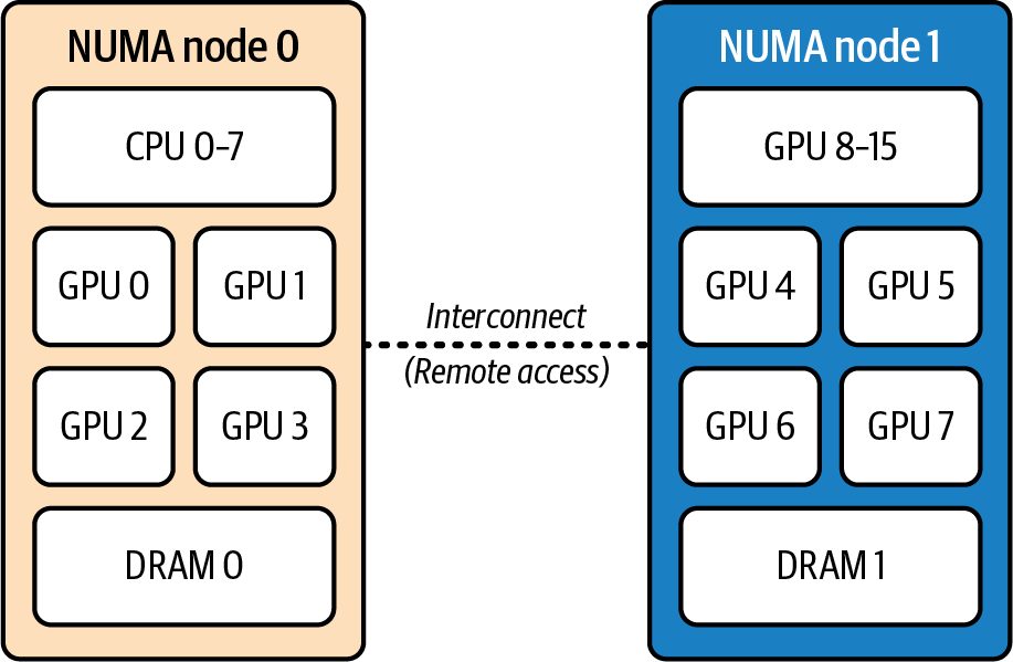
To explicitly specify NUMA-affinity, you need to “pin” processes or threads to spe‐ cific CPUs that are connected to the same NUMA node as the GPU. This type of CPU affinity is called CPU pinning. Suppose you have eight GPUs in a node, with four GPUs connected to NUMA node 0 and the other four to NUMA node 1. If you launch eight training processes, one per GPU, you should bind each training process to a CPU core—or set of CPU cores—connected to the same NUMA node as the GPUs. In this case, GPUs 0–3 are connected to NUMA node 0 and GPUs 4–7s are connected to NUMA node 1’s cores, as shown in Figure 3-4.
Figure 3-4. Eight GPUs in a node, with four GPUs connected to NUMA node 0 and the other four to NUMA node 1
This way, when a CPU process wants to feed data to GPU 4, it should be running on a CPU connected to NUMA node 1 since GPU 4 is connected to NUMA node 1. Linux provides tools to do this, including numactl --cpunodebind=<node> --membind= <node>, which launches a process pinned to the given NUMA node. You can also use taskset to pin processes to specific core IDs. Here is an example using numactl to bind the train.py script to a CPU running in the same NUMA node 1 as GPU 4: numactl --cpunodebind=1 --membind=1 \ python train.py --gpu 4
Configuring the CPUs and OS for GPU Environments | 63
This assumes we know the NUMA node ID and that we are binding the script to only
one GPU. Binding the train.py to multiple GPUs to an unknown NUMA node is a
bit more complicated. The following script dynamically queries the topology using
nvidia-smi topo and binds the script to GPUs using the local NUMA node:
     #!/bin/bash
     for GPU in 0 1 2 3; do
       # Query NUMA node for this GPU
       NODE=$(nvidia-smi topo -m -i $GPU \
              | awk '/NUMA Affinity/ {print $NF}')
       # Launch the training process pinned to that NUMA node
       numactl --cpunodebind=$NODE --membind=$NODE \
          bash -c "CUDA_VISIBLE_DEVICES=$GPU python train.py --gpu $GPU"
     done
Here, we use topo -m to get both CPU and NUMA affinities. We then extract the
single-node ID from the NUMA Affinity column. Finally, we bind both --cpunodebind
and --membind to that node to ensure your process’s threads and memory allocations
stay local to the GPU’s NUMA domain.
Many deep learning frameworks also let you set thread affinities programmatically.
For instance, PyTorch’s DataLoader exposes worker_init_fn so you can set CPU
affinity for each worker process during initialization, as shown here:
     import os
     import re
     import glob
     import subprocess
     import psutil
     import ctypes
     import torch
     import torch.distributed as dist
     from torch.nn.parallel import DistributedDataParallel as DDP
     from torch.utils.data import DataLoader, Dataset
     from functools import partial
     # Optional: NVML is preferred for GPU↔NUMA mapping
     try:
          import pynvml as nvml # pip install nvidia-ml-py3
          _HAS_NVML = True
     except Exception:
          _HAS_NVML = False
     # --- libnuma for memory binding
     _libnuma = ctypes.CDLL("libnuma.so")
     if _libnuma.numa_available() < 0:
         raise RuntimeError("NUMA not available on this system")
     _libnuma.numa_run_on_node.argtypes = [ctypes.c_int]
     _libnuma.numa_set_preferred.argtypes = [ctypes.c_int]
64 | Chapter 3: OS, Docker, and Kubernetes Tuning for GPU-Based Environments
def parse_physical_cpu_list(phys_str: str):
    """Parse '0-3,8-11' -> [0,1,2,3,8,9,10,11]."""
    cpus = []
    if not phys_str:
        return cpus
    for part in phys_str.split(','):
        part = part.strip()
        if not part:
            continue
        if '-' in part:
            start, end = map(int, part.split('-'))
            cpus.extend(range(start, end + 1))
        else:
            cpus.append(int(part))
    return cpus
def get_numa_cpus_for_node(node: int):
    """Read /sys/devices/system/node/node{node}/cpulist."""
    path = f"/sys/devices/system/node/node{node}/cpulist"
    with open(path, "r") as f:
        return parse_physical_cpu_list(f.read().strip())
def get_numa_cpus_and_memory():
    """Return (current_cpu_mask, preferred_node) from numactl --show."""
    out = subprocess.run(["numactl", "--show"],
        capture_output=True, text=True).stdout
    phys = re.search(r"physcpubind:\s*([\d,\-\s]+)", out).group(1)
    cpus = parse_physical_cpu_list(phys)
    node = int(re.search(r"preferred node:\s*(-?\d+)", out).group(1))
    return cpus, node
def get_gpu_numa_node(device: int) -> int:
    """
    Determine NUMA node for a GPU (prefer NVML; fall back to sysfs;
    final fallback to current preferred node).
    """
    # NVML path (preferred)
    if _HAS_NVML:
        try:
             nvml.nvmlInit()
             props = torch.cuda.get_device_properties(device)
             pci = props.pci_bus_id # '0000:03:00.0' or '00000000:03:00.0'
             # Normalize to 8-hex-digit domain if needed for NVML
             try:
                  domain, bus, devfn = pci.split(':')
                  if len(domain) < 8:
                      domain = domain.rjust(8, '0')
                  pci8 = f"{domain}:{bus}:{devfn}"
             except ValueError:
                 pci8 = pci
             try:
                  handle = nvml.nvmlDeviceGetHandleByPciBusId_v2(pci8)
Configuring the CPUs and OS for GPU Environments | 65
                      except AttributeError:
                          handle = nvml.nvmlDeviceGetHandleByPciBusId(pci8)
                      # Direct NUMA ID if driver exposes it
                      try:
                           numa_id = nvml.nvmlDeviceGetNUMANodeId(handle)
                          if isinstance(numa_id, int) and numa_id >= 0:
                               return numa_id
                      except Exception:
                          pass
                    # Derive from NVML CPU affinity
                    cpu_count = psutil.cpu_count(logical=True)
                    elems = (cpu_count + 63) // 64
                    mask = nvml.nvmlDeviceGetCpuAffinity(handle, elems)
                    cpus = []
                    for i, m in enumerate(mask):
                        m = int(m)
                        for b in range(64):
                             if m & (1 << b):
                                 cpu_id = i * 64 + b
                                 if cpu_id < cpu_count:
                                     cpus.append(cpu_id)
                    # Build CPU→NUMA map from sysfs and choose majority node
                    cpu2node = {}
                    for node_path in sorted(glob.glob("/sys/devices/system/node/node*")):
                         node_id = int(os.path.basename(node_path).replace("node", ""))
                         with open(os.path.join(node_path, "cpulist"), "r") as f:
                             for c in parse_physical_cpu_list(f.read().strip()):
                                 cpu2node[c] = node_id
                    counts = {}
                    for c in cpus:
                         n = cpu2node.get(c)
                         if n is not None:
                             counts[n] = counts.get(n, 0) + 1
                    if counts:
                         return max(counts.items(), key=lambda kv: kv[1])[0]
                except Exception:
                    pass
           # sysfs fallback
           try:
                props = torch.cuda.get_device_properties(device)
                pci = props.pci_bus_id
                sysfs_path = f"/sys/bus/pci/devices/{pci}/numa_node"
                with open(sysfs_path, "r") as f:
                     val = int(f.read().strip())
                     return val if val >= 0 else 0
           except Exception:
                pass
# last resort: current preferred node
66 | Chapter 3: OS, Docker, and Kubernetes Tuning for GPU-Based Environments
    _, node = get_numa_cpus_and_memory()
    return node if node >= 0 else 0
def set_numa_affinity(node: int):
    """Bind current process to CPUs and memory of the given NUMA node."""
    cpus = get_numa_cpus_for_node(node) # IMPORTANT: CPUs of target node
    psutil.Process(os.getpid()).cpu_affinity(cpus)
    _libnuma.numa_run_on_node(node)
    _libnuma.numa_set_preferred(node)
    print(f"PID={os.getpid()} bound to NUMA node {node} (CPUs={cpus})")
    return cpus
def _worker_init_fn(worker_id: int, node: int, cpus: list):
    """Reapply binding in each DataLoader worker (no CUDA calls here)."""
    psutil.Process(os.getpid()).cpu_affinity(cpus)
    _libnuma.numa_run_on_node(node)
    _libnuma.numa_set_preferred(node)
    print(f"Worker {worker_id} (PID={os.getpid()}) bound to NUMA node {node}")
 # ----- Example usage below -----
class MyDataset(Dataset):
    def __len__(self): return 1024
    def __getitem__(self, idx): return torch.randn(224*224*3, device='cpu')
def main():
    # DDP setup
    dist.init_process_group(backend="nccl", init_method="env://")
    device = torch.cuda.current_device()
    # Determine GPU's NUMA node and bind this process
    gpu_node = get_gpu_numa_node(device)
    cpus = set_numa_affinity(gpu_node)
    # Build dataloader with closure-based worker_init_fn
    dataset = MyDataset()
    init_fn = partial(_worker_init_fn, node=gpu_node, cpus=cpus)
    dataloader = DataLoader(
        dataset,
        batch_size=32,
        num_workers=4,
        pin_memory=True,
        persistent_workers=True, # reduces worker respawn churn
        worker_init_fn=init_fn,
        prefetch_factor=2,
    )
    # Model and DDP
    model = torch.nn.Linear(224*224*3, 10, bias=True).to("cuda")
    ddp_model = DDP(model, device_ids=[device], static_graph=True)
    for batch in dataloader:
        batch = batch.to("cuda", non_blocking=True)
Configuring the CPUs and OS for GPU Environments | 67
                out = ddp_model(batch)
                # ... loss, backward, optimizer ...
     if __name__ == "__main__":
         main()
This script binds the main training process and each DataLoader worker process to the GPU’s local NUMA node to prevent cross-NUMA memory access. In the DataLoader, we pass a closure-based worker_init_fn that reapplies the precomputed NUMA binding inside each worker. And we do this without touching any CUDA APIs in the worker. At startup, the process uses NVML to map the current GPU to its NUMA node and CPU-affinity mask. When available, we read the node directly via nvmlDeviceGet NUMANodeId. Otherwise, we derive it from the GPU’s CPU-affinity mask (nvmlDevice GetCpuAffinity). If NVML is unavailable or does not expose the node, we fall back to the kernel’s sysfs entry at /sys/bus/pci/devices/<PCI_ID>/numa_node. As a last resort, we use the process’s current preferred node. We then compute the CPU list for that node from /sys/devices/system/node/ node<N>/cpulist and apply CPU affinity to those cores with psutil. We also bind all future allocations to that node using libnuma (numa_run_on_node + numa_set_ preferred). Because some launchers, container runtimes, or kernels do not reliably propagate NUMA policy to children, we explicitly reapply and verify the binding in every forked worker. It’s not safe to rely on inheritance alone. Remember to set pin_memory=True and use non_blocking=True on H2D copies so that page-locked host buffers stay on the correct NUMA node. Prefer persis tent_workers=True to avoid re-forking workers and losing their affinity between epochs. And do not call torch.cuda.* in worker_init_fn. Instead, pass the GPU index using a closure or environment variable. The result is that data preparation and batch loading happen entirely in local mem‐ ory. This way, your GPUs stay busy and never need to pause for a remote‐NUMA hop. With this code, you get robust, topology‐aware affinity on any Linux server with libnuma and numactl installed. By default, numactl applies its CPU and memory policy to a process and is docu‐ mented to inherit that policy to all forked children. In practice, however, threads spawned by Python frameworks or exec’d subprocesses don’t always pick up the same settings on every kernel or Linux distribution. When using framework-managed worker processes, you should explicitly reassert the CPU and memory policy inside of each worker.
68 | Chapter 3: OS, Docker, and Kubernetes Tuning for GPU-Based Environments
               With a superchip architecture like Grace Blackwell (and Vera
               Rubin), the CPU and GPU are coherent using NVLink-C2C. How‐
               ever, Linux still models CPU DRAM and GPU HBM as separate
               pools. Binding CPU threads to the local CPU NUMA node still
               remains beneficial for locality.
In practice, pinning can eliminate unpredictable CPU scheduling behavior. It ensures that a critical thread such as a data-loading thread for your GPU doesn’t suddenly get migrated by the OS to a core on a different NUMA node in the middle of training or inferencing. In practice, it’s possible to see 5%–10% training throughput improve‐ ments just by eliminating cross-NUMA traffic and CPU core migrations. This also tends to reduce performance jitter and variance. Many high-performance AI systems evaluate CPU simultaneous multithreading (SMT), or hyperthreading as it’s often called—and sometimes disable it for more pre‐ dictable per-core performance, but the benefit is workload-dependent. These systems may also reserve a handful of cores exclusively for OS background tasks by setting the isolcpus kernel parameter to isolate them from the general scheduler. You can also use Kubernetes CPU isolation for system daemons. This ensures that the remaining cores are dedicated entirely to training and inference threads and doing useful work. It’s important to note that for integrated CPU-GPU superchips like NVIDIA’s Grace Blackwell, many of the traditional concerns about CPU-to-GPU data transfer are alle‐ viated because the CPU and GPU expose a coherent shared virtual address space over NVLink-C2C, while CPU DRAM and GPU HBM remain distinct memory pools. This means that issues like cross-NUMA delays are minimized, and the data can flow more directly between the CPU and GPU.
               It’s not a coincidence that NVIDIA tackled the CPU-to-GPU bot‐
               tleneck by combining the CPU and GPU onto a single superchip
               such as the Grace Blackwell architecture. In this design, the CPU
               and GPU even share a unified, coherent memory using NVLink-
               C2C at up to 900 GB/s, which minimizes data transfer overhead.
               Expect NVIDIA to continue addressing system bottlenecks with
               more of these types of hardware innovations codesigned with the
               needs of software and algorithms.
Even with the tightly coupled CPU-GPU superchip architecture, it’s still important to optimize the stack by ensuring that the hardware and software are configured prop‐ erly so that the integrated system operates at peak efficiency. Even in these tightly coupled architectures, you want to minimize any unnecessary delays in data handling to keep the GPU fully utilized. This includes configuring hugepages, using efficiency prefetching, and pinning memory, as you will see in the next sections.
Configuring the CPUs and OS for GPU Environments | 69
NUMA-Friendly Memory Allocation and Memory Pinning By default, a process will allocate memory from the NUMA node of the CPU it’s cur‐ rently running on. So if you pin a process to NUMA node 0, its memory will natu‐ rally come from NUMA node 0’s local RAM, which is ideal. However, if the OS scheduler migrates threads—or if some memory was allocated before you did the pinning—you could end up with the nonideal scenario in which a process running in NUMA node 0 is using memory from NUMA node 1. In this case, every memory access has to hop to the other NUMA node, negating the benefit of CPU pinning. To avoid this, the numactl --membind option forces memory allocation from a spe‐ cific NUMA node, as mentioned in an earlier section. In code, there are also NUMA APIs or even environment variables that can influence this configuration. The general rule is to keep memory close to the CPU, which is close to the GPU. That way the chain of data movement from memory to CPU to GPU is all within a single NUMA node. Here is the same example as before but with --membind=1 to force memory allocation from the preferred NUMA node that includes NUMA node 1: numactl --cpunodebind=1 --membind=1 python train.py --gpu 5 &
It’s important to note that when you launch a process under numactl, both its CPU (--cpunodebind) and memory policies (--membind) are applied to that process and inherited by all of its child processes. As such, any worker subprocesses forked by your training script will automatically use the same NUMA memory binding. How‐ ever, they must be created using a fork-based model. If you switch to a spawn start method, or otherwise exec a new program, those child processes do not inherit the parent’s memory policy. In addition, pinned memory, also called page-locked memory, is essential for efficient and direct GPU access. When memory is pinned, the OS won’t swap or move it. This leads to faster direct memory access (DMA) transfers. Copying data from pinned host memory to GPU can be 2–3× faster than from regular pageable memory since the GPU or NIC can perform DMA directly.
                     You can test the data-transfer bandwidth between CPU memory
                     and GPU memory using bandwidthTest --memory=<pinned or
                     pageable> from the installed CUDA utilities.
In fact, this is the basis of NVIDIA’s GPUDirect technologies such as GPUDirect RDMA, which allows NICs like InfiniBand to directly exchange data with GPU mem‐ ory. Similarly, GPUDirect Storage (GDS) allows NVMe drives to stream data into GPU memory without extra CPU overhead.
70 | Chapter 3: OS, Docker, and Kubernetes Tuning for GPU-Based Environments
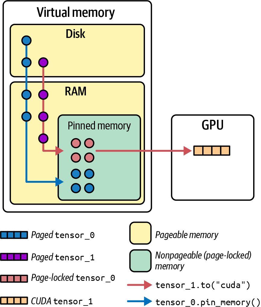
Deep learning frameworks provide options to use pinned memory for data loaders. For example, PyTorch’s DataLoader has a flag pin_memory=True, which, when true, means the batches loaded will be placed in pinned RAM, as shown in Figure 3-5.
Figure 3-5. Pinned memory (aka page-locked or nonpageable) is a type of memory that cannot be swapped out to disk
Memory pinning speeds up the tensor.to(device) operations because the CUDA driver doesn’t have to pin pages on the fly. It’s especially beneficial when you are using large batch sizes or reading a lot of data in each iteration. Many practitioners have noticed that just turning on pin_memory=True in PyTorch can improve performance up to 10%–20% by reducing data transfer bottlenecks and increasing host-to-device transfer throughput. In short, you should make sure that your data loader uses pinned memory (e.g., pin_memory=True in PyTorch DataLoader) and that GPUDirect RDMA and GDS are enabled for supported hardware. This will reduce data transfer latency. It’s important to note that the OS has a limit on how much memory a user can lock (pin). This is set with the ulimit -l <max locked memory> command. In container‐ ized environments, you can adjust the container’s security context and Docker --ulimit memlock setting accordingly. This way, the container can lock sufficient memory.
Configuring the CPUs and OS for GPU Environments | 71
                     If you plan to use large, pinned buffers, ensure the ulimit value is
                     high—or set it to unlimited. Otherwise the allocation might fail.
                     Typically, one sets it to unlimited for large AI workloads and high-
                     performance computing (HPC) applications.
Transparent Hugepages In addition to pinning memory and binding it to NUMA nodes, we should talk about transparent hugepages (THPs). Linux memory management typically uses 4 KB pages, but managing millions of tiny pages is inefficient when you have processes using tens or hundreds of gigabytes of memory, as in the case of deep learning data‐ sets, prefetched batches, model parameters, etc. Hugepages—2 MB or even 1 GB pages—can reduce the overhead of virtual memory management by making memory chunks bigger. The main benefits are fewer page faults and less pressure on the translation lookaside Buffer (TLB). The TLB is a cache that the CPU uses to map virtual addresses to physical ones. Fewer, larger pages means the TLB can cover more memory with the same number of entries, reducing misses. Hugepages typically produce modest gains—often on the order of ~3%–5% through‐ put improvement. They do this by reducing page-fault overhead and TLB pressure. Enabling THP is a simple win on most systems since the kernel will automatically back large allocations with 2 MB pages. In scenarios with very large memory pools (e.g., preallocated pinned buffers for I/O), you may also consider explicit hugepages using vm.nr_hugepages or hugetlbfs for more deterministic performance.
                     Remember that, when using large, pinned memory regions, you
                     should raise the ulimit -l setting (max locked memory) to a high
                     value or unlimited. If this limit is too low, your attempt to pin
                     memory can fail, leading to fallback on swappable memory—or
                     out-of-memory (OOM) errors.
It’s important to note that THP’s background compaction can introduce unpredicta‐ ble pauses that are disastrous for latency-sensitive LLM inference workloads. Linux is configured by default to use THP to automatically allocate 2 MB pages whenever pos‐ sible. This is often sufficient, but it’s worth testing for your workload. You can disable THP, but you will need to manually allocate and control hugepages. This will incur extra complexity, but it might be needed for low-latency workloads like inference. With THP disabled, your system will avoid stalls caused by kerneldriven defragmentations.
72 | Chapter 3: OS, Docker, and Kubernetes Tuning for GPU-Based Environments
               The modern consensus is to enable THP for most GPU-based
               training workloads in which throughput is important and to dis‐
               able THP completely (transparent_hugepage=never)—or use
               madvise—for workloads like inference in which latency is impor‐
               tant. This is also true for distributed training workloads in which
               many ranks (GPUs) allocate memory simultaneously.
Beyond CPU/memory pinning and hugepages, there are a few other OS-level tweaks worth mentioning. These include thread scheduling, virtual memory management, file‐ system caching, and CPU frequency settings, which we’ll cover in the next few sections.
Scheduler and Interrupt Affinity On a busy system, you want to make sure that important threads such as datapipeline threads aren’t interrupted frequently. Linux by default uses the Completely Fair Scheduler (CFS) that works well for most cases. But if you have a very latency-sensitive thread that feeds the GPU with data, for example, you could consider using real-time first in, first out (FIFO) or round-robin (RR) priority scheduling for that thread. This would make sure that the high-priority thread runs without being preempted by normal-priority threads. However, use this with caution, as real-time threads can starve other processes if not managed properly. In practice, however, if you’ve pinned your threads to dedicated cores, you often don’t need to mess with real-time thread priorities, but it’s worth keeping an eye on. Another option is to isolate cores or create separate CPU partitions to further reduce interruptions on these dedicated compute resources. To do this, you can use cset, kernel parameters like isolcpus and nohz_full, or cgroup cpuset isolation. With isolation, the OS scheduler leaves those CPU cores for you to use as you wish.
               cgroup CPU and memory affinity is strongly recommended in pro‐
               duction environments. Using these, each AI workload is isolated on
               its own physical cores and memory regions. This will prevent
               cross-workload contention and NUMA penalties. Tools like cpuset
               cgroups or container runtimes (docker --cpuset-cpus) should be
               used to enforce this.
You can assign each device’s hardware interrupts to cores on the same NUMA node. This will prevent cross-node interrupt handling that would otherwise incur extra latency and evict useful cache lines on a remote node. For example, if your GPU or NIC on NUMA node 0 raises an interrupt, you’d bind it to a core on node 0 so that no other node handles it. Without this binding, a CPU on a different NUMA node
Configuring the CPUs and OS for GPU Environments | 73
might process the interrupt. This would force cache coherency traffic and cross-node communication. In practice, performance-sensitive systems often disable the default irqbalance dae‐ mon or run it with bespoke rules. The other option is to manually set each interrupt’s affinity mask using /proc/irq/*/smp_affinity. By pinning every GPU and NIC interrupt to the nearest cores, you guarantee that those device interrupts are always serviced on the optimal NUMA node. In short, the combination of dedicated cores, appropriate scheduling priorities, and NUMA-aware hardware interrupt bindings can help minimize jitter for data loading threads that are feeding the GPUs.
Virtual Memory and Swapping It goes without saying, but you should always try to avoid memory swapping. If any part of your process’s memory gets swapped to disk, you will see a catastrophic, multiple-orders-of-magnitude slowdown. GPU programs tend to allocate a lot of host memory for data caching. If the OS decides to swap some data out of memory and onto disk, the GPU will experience huge delays when it needs to access that data. We recommend setting vm.swappiness=0, which tells Linux to avoid swapping except under extreme memory pressure. It effectively isolates your training job’s memory with cgroup limits to prevent any swapping.
                     You should use cgroups v2 through Docker or Kubernetes to pin
                     memory and CPUs to the AI process. This will enforce NUMA
                     affinity and no-swap policies in containerized environments.
You can also use sudo swapoff -a to temporarily disable all swap devices and files until the next reboot. Just make sure you have enough RAM for your workload—or put limits to prevent overcommit. Otherwise, the OOM killer may reap the process. Monitor swap usage using vmstat or free -m to make sure swap stays at zero. Another related setting is ulimit -l, as mentioned earlier for pinned memory. If you want to prevent memory from swapping, you should set that limit high or you may experience excessive memory swapping. Again, typically one sets this limit to unlimi‐ ted for large AI workloads that utilize a lot of memory.
74 | Chapter 3: OS, Docker, and Kubernetes Tuning for GPU-Based Environments
Filesystem Caching and Write-Back A best practice for large training jobs is to write frequent checkpoints to disk in case you need to restart a failed job from a known good checkpoint. During checkpoint‐ ing, however, huge bursts of data might fill up the OS page cache and cause stalls. For storage, you can adjust vm.dirty_ratio and vm.dirty_background_ratio to tune the page-cache size for buffering writes. For example, with multi-GB check‐ points, using a higher dirty ratio lets the OS batch more data in RAM before flushing to disk. This will smooth out large checkpoint writes and reduce stalls in your train‐ ing loop. Another option is to perform checkpointing in a separate thread. A more recent option in PyTorch is to write distributed checkpoint partitions from nodes across the cluster. In this case, the checkpoint partitions will be combined when the checkpoint is loaded after a failed-job restart. In latency-sensitive training workflows, it’s best to bypass the page cache entirely. For example, open checkpoint files with O_DIRECT or use Linux’s io_uring for asynchro‐ nous I/O to avoid page-cache stalls. After writing each checkpoint, call posix_fadvise (fd, 0, 0, POSIX_FADV_DONTNEED) to immediately drop those pages from cache and prevent memory pressure on subsequent iterations.
CPU Frequency and C-states By default, many compute nodes will run CPUs in a power-saving mode, which either downclocks a CPU or puts it to sleep when it’s idle. This helps save energy and reduce heat and lowers the cost. During model training, the CPUs might not always be 100% utilized as the GPUs are churning through the final batches of their dataset. However, these power management features could cause extra latency when the system wakes the CPUs up again when new work arrives. For maximum and consistent performance, AI systems often configure the CPU fre‐ quency governor to “performance” mode, which keeps the CPU at max frequency all the time. This can be done using cpupower frequency-set -g performance or in the Basic Input/Output System (BIOS). Likewise, disabling deep C-states can keep cores from going into a low-power sleep state. CPU C-states are power-saving modes defined by the system’s ACPI specifica‐ tion. When a CPU core is idle, it can enter a C-state to save energy. The deeper the Cstate, the more power is saved but the longer it may take for the core to wake up when work arrives. Disabling deeper C-states can remove excessive latency spikes. C0 is active; everything above C0 represents a deeper state of sleep.
Configuring the CPUs and OS for GPU Environments | 75
                     In practice, many server BIOS/UEFI (Unified Extensible Firmware
                     Interface) offer a high-performance profile that automatically sets
                     the CPU governor to “Performance” and disables deep C-states.
Essentially, we can trade a bit of extra power draw for more responsive CPU behavior. In a training scenario where GPUs are the big power consumers, a bit more CPU power usage is usually fine if it keeps the GPUs fed. For example, if a data loader thread sleeps while waiting for data and the CPU goes into the deep C6 state, signifi‐ cant portions of the CPU are powered down to maximize energy savings. If the CPU enters a deeper sleep state, it might take a few microseconds to wake up. While this is not a long time, many microseconds can add up and can cause GPU bubbles if not managed properly. Bubbles are periods of time when the GPU is wait‐ ing for the CPU to resume data processing. By keeping the CPU ready, we reduce such hiccups. Many BIOSes for servers have a setting to disable C-states—or at least limit them.
                     You should always turn off anything in your system that might
                     introduce unpredictable latency, such as excess context switching,
                     CPU frequency scaling, and memory-to-disk swapping. The result
                     should be that your CPUs deliver data to the GPUs as fast as the
                     GPUs can consume it, without the OS scheduling things on the
                     wrong core or taking CPU cycles away at the wrong time.
Tune Host CPU Memory Allocator On a well-tuned GPU server, CPU usage may not be very high since GPUs handle most of the computation. However, CPU usage should remain steady and in lockstep with GPU activity. The CPUs must stay busy preparing each incoming batch while the current batch is being processed by the GPU. Proper CPU‐to‐GPU handoff is crucial for sustaining high GPU utilization. By tun‐ ing your host’s memory allocator (jemalloc or tcmalloc), you can eliminate unpre‐ dictable pauses in data preparation. This will keep GPUs running at their peak— except for intentional synchronization points. After tuning, you should see each GPU’s utilization hover near 100% and drop only at required synchronization barriers. The GPUs should never stall for data due to CPUside delays. With jemalloc, you can shard allocations into per-CPU arenas (narenas), enable background_thread for off-path purging, and lengthen dirty_decay_ms/muzzy_decay_ms so that freed pages aren’t immediately returned to the OS. This will minimize lock contention and fragmentation.
76 | Chapter 3: OS, Docker, and Kubernetes Tuning for GPU-Based Environments
You can tune jemalloc with the MALLOC_CONF environment variable as follows:
    export MALLOC_CONF="narenas:8,dirty_decay_ms:10000,muzzy_decay_ms:10000
    ,background_thread:true"
Similarly, tcmalloc benefits from tuning the TCMALLOC_MAX_TOTAL_THREAD_ CACHE_BYTES and TCMALLOC_RELEASE_RATE environment variables. These will provide larger per-thread caches so that small allocations avoid global locks and syscalls— keeping CPU threads ready to feed the GPU with low, predictable latency. You can do this as follows: export TCMALLOC_MAX_TOTAL_THREAD_CACHE_BYTES=$((512*1024*1024)) export TCMALLOC_RELEASE_RATE=16 In short, optimizing the allocator can reduce allocator overhead and fragmentation. This will keep CPU threads consistently fast and avoid unexpected stalls feeding the GPU. Experiment with these environment variables and tune them for your specific workload and environment.
GPU Driver and Runtime Settings for Performance We’ve optimized the CPU side, but there are also important settings for the GPU driver and runtime that can affect performance—especially in multi-GPU and multi‐ user scenarios. NVIDIA GPUs have a few knobs that, when tuned properly, can reduce overhead and improve how multiple workloads share a GPU. Next, we’ll cover GPU persistence mode, the partitions of MPS, MIG, and a few other considerations like clock settings, ECC memory, and out-of-memory behavior.
GPU Persistence Mode By default, if no application is using a GPU, the driver may put the GPU into a lowerpower state and unload some of the driver’s context. The next time an application comes along and wants to use the GPU, there’s a cost to initialize it. This can take on the order of a second or two for the driver to spin everything up. GPU initialization overhead can negatively impact performance for workloads that periodically release and reacquire the GPU. For instance, consider a training cluster where jobs are starting and stopping frequently. Or a low-volume inference cluster that has to wake up the GPU every time a new inference request arrives. In both of these cases, the overhead will reduce overall workload performance. Persistence mode is enabled by running the nvidia-persistenced daemon. This keeps the GPU driver loaded and the hardware in a ready state even when no applica‐ tion is active. This requests that the system not fully power down the GPU when idle, which prevents power gating. Persistence keeps the GPU awake so that the next job has zero startup delay. This is generally recommended for long-running and
GPU Driver and Runtime Settings for Performance | 77
latency-sensitive workloads. You can enable the persistence daemon at boot time using the following command: systemctl enable nvidia-persistenced
                     In Kubernetes environments, the NVIDIA GPU Operator can be
                     configured to enable persistence mode on all GPUs automatically.
On AI clusters, it’s common to just enable persistence mode on all GPUs at server boot time. This way, when a job begins, the GPUs are already initialized and can start process‐ ing immediately. It won’t make your actual compute any faster, as it doesn’t speed up the math operations, but it shaves off job-startup latency and prevents cold start delays. GPU persistence mode also helps with interactive usage, as without persistence, the first CUDA call you make after some idle time might stall while the driver reinitial‐ izes the GPU. With persistence on, that call returns quickly. The only downside of persistence is a slightly higher power draw when idle since the GPU stays in a higher readiness state. But, for most data center GPUs, this is an acceptable trade-off for better performance consistency. Once GPU persistence mode is set by an admin with sudo access, you can enjoy the benefits and move on to tackle other optimizations.
MPS Normally, when multiple processes share a single GPU, the GPU’s scheduler timeslices between them. For example, if two Python processes each have some kernels to run on the same GPU, the GPU might execute one process’s kernel, then the other process’s kernel, and so on. If those kernels are short and there’s an idle gap between them, the GPU can end up underutilized as it’s doing “ping-pong” context switches and not overlapping the work. NVIDIA’s MPS is a feature that creates a sort of umbrella under which multiple pro‐ cesses can run on the GPU concurrently and without strict time-slicing. With MPS, the GPU can execute kernels from different processes at the same time as long as the GPU resources (streaming multiprocessors [SMs], Tensor Cores, etc.) are available. MPS essentially merges the contexts of the processes into one scheduler context. This way, you don’t pay the full cost of switching and idling between independent processes. When is MPS useful? For model training, if you normally run one process per GPU, you might not use MPS. But if you have scenarios like running many inference jobs on one big GPU, MPS is a game changer. Imagine you have a powerful GPU or GPU cluster, but your inference job—or set of multiple inference jobs—doesn’t fully use it.
78 | Chapter 3: OS, Docker, and Kubernetes Tuning for GPU-Based Environments
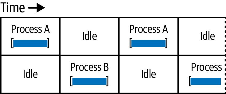
For instance, consider running four separate inference jobs on one 40 GB GPU, each using 5–10 GB and only 30% of GPU compute. By default, each inference job gets a time-slice, so at any moment, only one job’s work is actually running on the GPU. That leaves the GPU 70% idle on average. If you enable MPS for these inference jobs, the GPUs can interleave their work so that while one job is waiting on memory, another job’s kernel might fill the GPU, etc. The result is higher overall GPU utilization. In practice, if two processes each use 40% of a GPU, with MPS you might see the GPU at 80%–90% utilization serving both. For instance, two training processes that each would take one hour on their own—on the same GPU, running sequentially—can run together with MPS and finish in a bit over one hour total in parallel instead of two hours sequentially. For instance, two training processes that each would take one hour on their own—on the same GPU, running sequentially—can run together with MPS. In this case, they would finish in a bit more than one hour total in parallel instead of two hours sequentially. The speedup from MPS can approach a near-doubling when kernels and memory band‐ width from concurrent clients complement one another. To visualize, imagine Pro‐ cess A and Process B each launching kernels periodically without MPS. The GPU schedule might look like A-B-A-B with gaps in between while each one waits, as shown in Figure 3-6.
Figure 3-6. GPU alternates between running Process A’s kernels and Process B’s kernels and creates idle gaps in which one process is waiting while the other is active
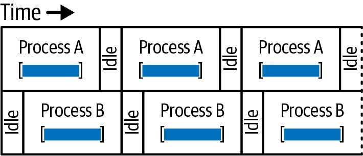
With MPS, the schedule overlaps A and B so that whenever A isn’t using some parts of the GPU, B’s work can use them simultaneously, and vice versa. This overlapping eliminates idle gaps, as shown in Figure 3-7.
Figure 3-7. Reducing idle gaps for processes A and B using MPS
GPU Driver and Runtime Settings for Performance | 79
Setting up MPS involves running an MPS control daemon (nvidia-cuda-mpscontrol), which then launches an MPS server process that brokers GPU access. On modern GPUs, MPS is more streamlined as clients (the processes) can talk directly to the hardware with minimal interference from the compute node itself. Typically, you start the MPS server on a node—often one per GPU or one per user— and then run your GPU jobs with an environment variable that connects them to MPS. All jobs under that server will share the GPU concurrently. Another feature of MPS is the ability to set an active thread percentage per client. This limits how many SMs (GPU cores, essentially) a client can use. This can be use‐ ful if you want to guarantee quality of service (QoS) where two jobs, for example, each get at most 50% of the GPU’s execution resources. In this case, you can set CUDA_MPS_ACTIVE_THREAD_PERCENTAGE=50 to cap a client to about 50% of SM execu‐ tion capacity. If not explicitly set, the jobs will just compete and use whatever GPU resources they can. Note that MPS does not partition GPU memory, so all processes will share the full GPU memory space. MPS is mainly about compute sharing and scheduling. The issue is that one process could request a massive amount of GPU RAM, cause an OOM error on the GPU, and result in terminating all of the other processes running on the GPU. This is very disruptive. Also, if one program saturates the GPU 100% on its own, MPS won’t magically make it go faster, as you can’t exceed 100% utilization. It’s beneficial only when individual jobs leave some slack that others can fill. Another limitation of MPS is that, by default, all MPS clients must run as the same Unix user since they share a context. In multiuser clusters, this means MPS is usually set up at the scheduler level such that only one user’s jobs share a GPU at a time. Otherwise, you can configure a system-wide MPS that’s shared by all users, but understand that the jobs are not isolated from a security standpoint. Modern NVIDIA drivers support multiuser MPS so that processes from different Unix users can share a single MPS server. This improves usability but does not pro‐ vide memory isolation. Prefer MIG when strong isolation is required. One specific alternative to MPS is a feature for time-slicing GPUs in Kubernetes. Time-slicing on Kubernetes allows the device plugin to schedule different pods on the same GPU by time. For instance, if you configure a single GPU with a time-slicing replication factor of four, four pods on that GPU can each receive a time share. Kubernetes time-slicing is sort of an automated time-sharing algorithm that doesn’t require MPS. However, this doesn’t overlap execution. Instead, it just switches more rapidly than the default driver would. Time-slicing may be useful for interactive workloads where you prefer isolation at the cost of some idle time. For highthroughput jobs, overlapping with MPS or splitting the GPU with a MIG is usually better than fine-grained time-slicing, as discussed next.
80 | Chapter 3: OS, Docker, and Kubernetes Tuning for GPU-Based Environments
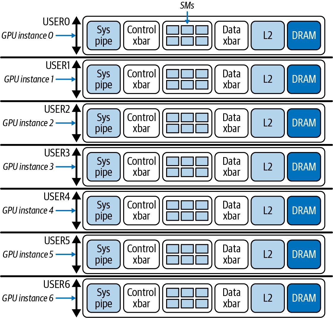
MIG Modern GPUs can be partitioned at the hardware level into multiple instances using MIG. MIG is a form of virtualization but done in hardware. This way, the overhead is very low—maybe a few percent—due to the loss of some flexibility. If one instance is idle, it can’t lend its resources to another, as they are hard parti‐ tioned. MIG allows a GPU to be sliced into as many as seven smaller logical GPUs— each with its own dedicated portion of memory and compute units, or SMs, as shown in Figure 3-8.
Figure 3-8. Seven MIG slices on a modern GPU
By convention, NVIDIA’s MIG profile naming uses the prefix <X>g to denote the number of compute slices between 1 (min) and 7 (max) on modern GPUs. Each slice number represents a number of SM groups allocated to that partition. Each SM group is roughly a 1/7 slice of the total number of SMs. If a GPU has 132 SMs, each 1/7 slice represents 132 SMs × 1/7 = ~19 SMs in a group. As such, 1g represents ~19 SMs, 2g represents ~38 SMs, all the way up to 7g, which represents the total of ~132 SMs.
GPU Driver and Runtime Settings for Performance | 81
In contrast, and somewhat confusingly, the suffix <Y>gb specifies the exact amount of HBM GPU RAM in gigabytes that is reserved for that profile. The MIG profile values are fixed for each GPU generation and type and listed in the NVIDIA documenta‐ tion. For the Blackwell B200, some of the MIG profile values are shown in Table 3-1.
Table 3-1. MIG Profiles for Blackwell B200 (source: https://oreil.ly/FsPEx) Profile name Fraction of memory Fraction of SMs L2 cache size Copy engines Number of instances MIG 1g.23gb 1/8 1/7 1/8 2 7 MIG 1g.45gb 2/8 1/7 2/8 2 4 MIG 2g.45gb 2/8 2/7 2/8 3 3 MIG 3g.90gb 4/8 3/7 4/8 6 2 MIG 4g.90gb 4/8 4/7 4/8 8 1 MIG 7g.180gb Full Full Full 16 1
The table also shows the number of hardware units, copy engines, and L2 cache frac‐ tions for each profile. These fixed profiles align with the GPU’s hardware memory controllers such that each memory slice maps to contiguous HBM channels. This two-part scheme separates compute capacity (number of SM groups) from memory capacity (total GB). Administrators can choose combinations of MIG pro‐ files. The sum of allocated SMs and HBM does not need to exactly match the full GPU capacity. However, certain combinations are constrained by hardware partition‐ ing. They cannot invent new slice sizes, for instance. Administrators can enable or disable only the supported MIG profiles (e.g., 1g.23gb, 2g.45gb, 4g.90gb, etc.) on each GPU using tools like nvidia-smi -mig or using the NVIDIA Kubernetes GPU Operator’s nvidia.com/mig.config config map. Reconfi‐ guring MIG requires draining workloads and invoking MIG’s dynamic reconfigura‐ tion capability to apply the changes. Once a GPU is in MIG mode, modern GPUs can create and destroy MIG partitions dynamically without rebooting the entire system. You can adjust MIG instances on the fly after draining existing workloads, but to enable or disable MIG mode itself on a GPU, a reset of that GPU is needed. Each MIG instance acts like a separate GPU from the perspective of software since it has its own memory, its own SMs, and even separate engine contexts. The benefit of MIG is strong isolation and guaranteed resources for each job. If you have multiple users or multiple services that need only, say, 10 GB of logical GPU memory each, you can pack them onto one physical GPU without them interfering with one anoth‐ er’s memory or compute.
82 | Chapter 3: OS, Docker, and Kubernetes Tuning for GPU-Based Environments
Jobs can request MIG devices specifically, but you have to be careful to schedule in a way that uses all slices. For instance, if you have a 7-slice setup and a job takes only 1 slice, the other 6 should be packed with other jobs, or you’re leaving a lot idle. It’s pos‐ sible to configure certain nodes in your cluster to use MIG for small inference jobs, for example, and configure other nodes for non-MIG workloads for large training jobs. One important operational note is that, in order to use MIG, you typically configure it at the system level—or at least at the node level. The GPU has to be put into MIG mode, the slices created, and the GPU reset. Once these happen, the slices appear as separate devices to the system—each with their own unique device ID. If you’re not using all of the available MIG slices because of poor upfront planning, you’ll end up wasting resources by leaving them fragmented and unused. It’s impor‐ tant to plan partition sizes upfront to match your workloads—and adjust the parti‐ tion sizes when the workload changes. You will need to reset the GPUs to pick up the change. For large-scale model training jobs and inference servers that span many GPUs, MIG is typically not useful since we want access to the full set of GPUs. On the other hand, for multitenant, small-model inference servers that can run smaller GPU partitions, MIG and its isolation features could be useful.
                As of this writing, when a GPU is in MIG mode, GPU-to-GPU
                peer-to-peer communication (including NVLink) is disabled. This
                applies to both NVLink and PCIe P2P across GPUs. MIG instances
                cannot engage in P2P with other GPUs. CUDA IPC across MIG
                instances is also limited. This can reduce distributed training
                throughput. Confirm that your training or inference topology does
                not rely on GPU peer paths before enabling MIG. Large-scale
                training jobs (and sparse MoE expert inference systems) require
                massive GPU-to-GPU communication and are typically not good
                candidates for MIG. Communication between GPU MIG instances
                must travel through either the host or network fabric.
In short, enable MIG only when you need to run multiple independent jobs on the same GPU with strong isolation. Do not use MIG for large-scale distributed training or inferencing that spans GPUs, as you want access to the full power of the GPUs and their fast interconnects. In our context of large transformer-based model training and inferencing, we will leave MIG off. But it’s good to know that this feature exists. Perhaps a cluster might dynamically switch modes and run MIG during the day when lots of small training or inferencing experiments are happening, then turn MIG off at night to run big train‐ ing jobs that use whole GPUs.
GPU Driver and Runtime Settings for Performance | 83
                     The Kubernetes device plugin will list MIG devices as resources
                     like nvidia.com/mig-1g.23gb in the case of a 1/7 GPU slice with a
                     total 23 GB for the slice.
GPU Clock Speeds and ECC NVIDIA GPUs have something called GPU Boost, which automatically adjusts the core clock within power and thermal limits. Most of the time, you should let the GPU just do its thing. But some users like to lock the clocks for consistency so that the GPU always runs at a fixed maximum frequency. This way, run-to-run performance is stable and not subject to variations in power or temperature. Fixing the clock is extremely important when performing benchmarks since later runs may be throttled due to excessive heat. If you do not account for this, you may inadvertently interpret the poor results of later runs incorrectly since the GPUs of these subsequent runs may be throttled due to excessive heat caused by previous runs. Specifically, NVIDIA’s GPU Boost will vary the core clock up or down to stay within power/thermal limits. Locking the clock at the max stable frequency using nvidiasmi -lgc to lock the core clock and -ac to lock the memory clock. This will make sure the GPU runs at a constant frequency—and prevents the GPU’s Boost default functionality from downclocking in later runs.
                     This is mostly relevant during benchmarking to achieve determin‐
                     istic and reproducible results. For everyday training and inferenc‐
                     ing, it’s recommended to leave auto-boost on unless you notice
                     significant performance variance and GPU throttling.
Locking the clocks is something to be aware of if you’re chasing the last bit of deter‐ minism and consistency. Typically, however, leaving the GPU in the default autoboost mode is fine. Some teams purposely underclock the GPUs to reduce heat—especially if they are running very long jobs and don’t want to suffer the eventual thermal slowdown over time. Data center GPUs typically have enough temperature headroom—as well as proper air and liquid cooling—so that you don’t need to do this, but it’s good to know that it’s an option. Another approach is to use nvidia-smi -pl to set a power limit slightly below the maximum thermal design power (TDP) of the GPU. TDP is the maximum amount of heat, measured in watts, that a GPU can generate under sustained load. This dictates the amount of heat that must be dissipated to prevent overheating.
84 | Chapter 3: OS, Docker, and Kubernetes Tuning for GPU-Based Environments
If you set the power limit below TDP, the GPU Boost will auto-adjust clocks below the thermal throttle point. This can reduce peak heat generation, prevent throttling, and incur minimal performance impact. ECC memory on GPUs is another consideration. ECC ensures that if there’s a singlebit memory error caused by cosmic rays, for example, the memory can be corrected on the fly. And if there’s a double-bit error, the error is detected and will throw an error to the calling code. ECC is usually enabled by default on NVIDIA data center GPUs. Disabling ECC can free up a small amount of memory since ECC requires extra bits for error checking. This might yield a marginal performance gain by reducing the overhead associated with on-the-fly error checking, but typically just a few percent. However, turning off ECC also removes critical memory-error protection, which can lead to system instability or undetected data corruption. For NVIDIA’s data center GPUs, including Hopper and Blackwell, ECC comes enabled by default and is intended to remain enabled to ensure reliable, errorcorrected computation and data integrity. For long training or inference jobs on huge models, a single memory error could crash the job completely or, even worse, silently corrupt your model without a warning. It’s recommended to always keep ECC on for any serious AI workload. The only time you’d possibly consider turning it off is in a research setting where you are fine with taking the risk because you need that extra sliver of memory for your model to fit into your limited-memory GPU cluster. Toggling ECC mode requires resetting the GPU and likely restarting jobs that are currently running on that GPU. So it’s not a toggle that you want to switch frequently. Keep ECC on for stability and reliability. The peace of mind outweighs the negligible speedup of turning ECC off.
GPU Memory Oversubscription, Fragmentation, and Out-of-Memory Handling Unlike CPU RAM, by default there is no such thing as GPU “swap” memory. If you try to allocate more GPU memory than available, you will get an unfriendly OOM error along with an even-unfriendlier process crash. There are a couple of mecha‐ nisms to mitigate this issue: allow memory to grow dynamically, embrace unified memory across CPU and GPU, and utilize memory pools and caching allocators. By default, some frameworks (e.g., TensorFlow) grab all of the available GPU mem‐ ory at startup to avoid fragmentation and improve performance. If you don’t know this, it can be very bad in scenarios where you are sharing the GPU. PyTorch, by default, allocates GPU memory only as needed.
GPU Driver and Runtime Settings for Performance | 85
TensorFlow has an option (TF_FORCE_GPU_ALLOW_GROWTH=true) to make it start small and dynamically grow the GPU memory usage as needed—similar to PyTorch. How‐ ever, neither PyTorch nor TensorFlow lets you allocate more memory than the GPU has available. But this lazy allocation plays nicer in multitenant scenarios because two processes won’t both try to simultaneously allocate the maximum available GPU memory from the start. CUDA’s Unified Memory system lets you allocate memory without predefining whether it resides on the CPU or GPU. The CUDA Runtime handles moving pages as needed. Modern NVIDIA GPUs like Hopper and Blackwell include hardware support for on-demand paging using the Page Migration Engine (PME). PME automatically migrates memory pages between GPU memory and host CPU RAM when the GPU runs low on available memory. However, while PME provides flexibility, relying on it can introduce performance penalties compared to having enough GPU memory for your workload. This GPU-to-CPU memory offloading can be slow, however, since CPU memory I/O is slower than GPU high-bandwidth memory (HBM) I/O, as we learned in Chapter 2. This mechanism is mostly a convenience for practitioners trying to run models that don’t fit into GPU RAM. For performance-critical workloads, you generally want to avoid relying on unified memory oversubscription where possible. It’s there as a safety net instead of outright crashing your script, but your job will run slower when GPU memory is oversubscribed. Libraries like PyTorch use a caching allocator so that when you free GPU memory, it doesn’t return the memory to the OS immediately. Instead, it keeps it to reuse for future allocations. This avoids memory fragmentation and the overhead of asking the OS to repeatedly allocate the same block of memory. You can configure PyTorch’s allocator using environment variables like PYTORCH_ALLOC_CONF (formerly PYTORCH_CUDA_ALLOC_CONF) to set a max pool size. We’ll cover optimizations to PyTorch’s memory-allocation mechanism in a later chapter. If you run into the GPU OOM error, which you surely will at some point, it’s likely caused by memory fragmentation or excessive memory caching. You can try to clear the cache using PyTorch’s torch.cuda.empty_cache(), but it almost always means your workload legitimately needs that much memory. PyTorch also provides tools like torch.cuda.memory_stats() and torch.cuda.mem ory_summary() to help diagnose fragmentation by showing allocated versus reserved memory. NVIDIA’s Nsight Systems also shows GPU memory usage patterns to help identify memory leaks, long-lived allocations that correlate with leaks, CPU-GPU
86 | Chapter 3: OS, Docker, and Kubernetes Tuning for GPU-Based Environments
interconnect activity, and GPUDirect Storage timeline tracing. Additionally, the Nsight Compute profiler provides low-level kernel analysis, including occupancy, throughput, and NVLink usage. We’ll cover all of these in the upcoming chapters. Docker provides the --gpus flag to select and expose GPUs to a container, but it does not support setting a GPU memory limit. If you need hard isolation for GPU mem‐ ory or compute, use MIG to partition the device or use Multi-Process Service (MPS) with active thread percentage for fair sharing. Configure limits in Kubernetes using MIG resources like nvidia.com/mig-2g.45gb when you require strict partitioning. In multitenant nodes, this could be useful to isolate jobs. In a single-job-per-GPU sit‐ uation, it’s not common to set a memory limit, as you want to let the job use as much of the GPU memory as it can get. In general, running out of GPU memory is something you can manage at the applica‐ tion level. For instance, you can reduce the data batch size, model weight precision, or even the model parameter count, if that’s an option. A best practice is to monitor GPU memory usage with nvidia-smi or NVML APIs during model training and inferencing. If you’re close to the memory limit, consider workarounds like reducing batch size, using activation checkpointing for training, or other techniques to lower memory usage. Also, you should ensure that your CPU memory isn’t being swapped, as this would indirectly hurt your GPU utilization and goodput because each time your GPU tries to fetch something from the CPU host, but the host memory page has been swapped to disk, your performance will be bottlenecked by the much slower disk I/O. So it’s important to combine these memory-reduction best practices with the earlier advice about pinning memory, increasing the ulimit, and disabling swappiness, etc. In short, it’s recommended to always keep the GPU driver loaded instead of unload‐ ing the GPU driver between jobs. This is similar to GPU persistence mode but at a deeper level. Some clusters are configured to unload the driver when no jobs are run‐ ning in order to free OS kernel memory and for security. However, if you do that, the next job has to pay the cost of reloading the GPU driver and, if MIG is used, reconfi‐ guring MIG slices.
               It’s recommended to keep the driver and any MIG configuration
               persistent across jobs. The only time you want to unload the GPU
               driver is for troubleshooting or upgrading the driver. As such, clus‐
               ter admins often set up the system so that the NVIDIA driver mod‐
               ules are always present once the machine boots.
GPU Driver and Runtime Settings for Performance | 87
Container Runtime Optimizations for GPUs Many AI systems use orchestration tools and container runtimes to manage the soft‐ ware environment. Kubernetes and Docker are popular in AI infrastructure. Using containers ensures that all dependencies, including CUDA and library versions, are consistent. This avoids the “but it works on my machine” problem. Containers intro‐ duce a bit of complexity and a tiny amount of overhead, but with the right configura‐ tion, you can get near bare-metal performance for GPU workloads using containers. A container running on a node is not a traditional virtual machine (VM). In contrast to VMs, containers share the host OS kernel so that CPU and memory operations perform at near-native speed. And with the NVIDIA Container Toolkit, GPU access from within a Docker container is direct and does not incur overhead.
                     For modern GPUs running with the latest NVIDIA Container
                     Toolkit, GPU performance within a properly configured environ‐
                     ment is virtually identical (< 2% difference) to running the code
                     directly on the bare-metal host outside of the container. In fact,
                     Red Hat OpenShift and Kubernetes were used in the MLPerf Infer‐
                     ence v5.0 results, which demonstrates that modern containers and
                     orchestration configuration do not compromise efficiency or
                     latency.
NVIDIA Container Toolkit and CUDA Compatibility One challenge when using containers with GPUs is making sure that the CUDA libraries inside the container match the driver on the host. NVIDIA solves this through their Container Toolkit and base Docker images. The host provides the NVI‐ DIA driver, which, remember, is tightly integrated with the kernel and hardware. Inside the container, you typically find the CUDA runtime libraries of a certain version. The general rule is that the host’s NVIDIA driver version must be at least as recent as the minimum driver version required by the CUDA version inside the container. For CUDA 13.x, the minimum required Linux host driver branch is R580 or newer. For CUDA 12.x, the minimum required Linux host driver branch is R525 or newer. Using a newer CUDA runtime with an older driver will cause the CUDA initialization to fail.
                     Each new CUDA version requires a minimum NVIDIA driver ver‐
                     sion. Always consult NVIDIA’s official compatibility matrix and
                     upgrade the host driver when you update the CUDA toolkit.
88 | Chapter 3: OS, Docker, and Kubernetes Tuning for GPU-Based Environments
For Docker and Kubernetes environments, the simplest approach is to use NVIDIA’s official base Docker images from the NVIDIA GPU Cloud (NGC) or DockerHub image repositories. These images (e.g., nvcr.io/nvidia/pytorch or similar) bundle the proper versions of the CUDA runtime, cuDNN, NCCL, etc. In addition, these Docker images list the minimum required CUDA driver, depending on the CUDA version. This way, you get support for the latest hardware without dependency headaches.
NVIDIA Container Runtime Alternatively, NVIDIA’s container runtime can actually inject the host driver libraries into the container at runtime, so you don’t even need to ship the NVIDIA driver inside the image. Instead, you just rely on the host’s driver. Again, this works because the container isn’t fully isolated like a traditional VM. Docker containers are allowed to use host devices, volumes, and libraries. Inside the container, your application uses the CUDA runtime libraries, such as libcudart.so from the container image, while the NVIDIA Container Toolkit injects the host’s driver libraries such as libcuda.so and libnvidia-ml.so at container start. The host driver libraries are invoked directly on the host so that everything just works. The split between CUDA runtime libraries (container) and NVIDIA Container Tool‐ kit (host) is supported as long as the host driver meets the minimum version required by the CUDA Toolkit in the image. If you were to mismatch and try to use a newer CUDA version in the container with an old driver on the host, you’d likely get an error. It’s important to match the CUDA and driver versions. The key takeaway is that there is no hypervisor or virtualization layer involved when using containers for GPUs. The container is sharing the host kernel and driver directly, so when a kernel launches on the GPU, it’s as if it launched from the host. In other words, you aren’t losing performance to Docker-based virtualization—unless you are using something like VMware or Single Root Input/Output Virtualization (SR-IOV) virtual GPUs, which is a special scenario that requires some tuning. With Docker plus NVIDIA, it’s basically the equivalent of bare metal performance.
               The NVIDIA Container Toolkit works with containerd and Pod‐
               man as well, not only Docker. This is relevant for modern Kuber‐
               netes environments that use containerd as the default container
               runtime.
Container Runtime Optimizations for GPUs | 89
Avoiding Container Overlay Filesystem Overhead The main difference when running in a Docker container versus running directly on the host might be in I/O. Containers often use a union filesystem that transparently overlays multiple underlying filesystems, like the host filesystem and the container filesystem, into a single, unified view. In a union filesystem such as OverlayFS, files and directories from multiple sources will appear as if they belong to one filesystem. This mechanism is especially useful for containers, where the read-only filesystem from the base image layer is combined with a writable container layer. There is some overhead when using an overlay filesystem, however. This extra latency arises because the filesystem must check multiple underlying layers—both read-only and writable—to determine which version of a file should be returned. The additional metadata lookups and the logic for merging these layers can add a small amount of overhead compared to reading from a single, simple filesystem. Furthermore, there is overhead when writing to the copy-on-write (CoW) mecha‐ nism used by the overlay. CoW means that when you modify a file in the read-only layer (e.g., the base image), the file must first be copied to the writable layer. The write then happens to the copied writable file—instead of the original, read-only file. As mentioned earlier, reading a modified file requires looking at both the read-only and writable layers to determine which is the correct version to return. Model training often involves heavy I/O operations when reading datasets, loading a model, and writing model checkpoints. To work around this, you can mount a host directory—or network filesystem—into the container using bind mounts. Bind mounts bypass the overlay and therefore perform similarly to disk I/O directly on the host. If the host filesystem is something like an NVMe SSD or an NFS mount, you get the full performance of that underlying storage device. We purposely do not package a multi-terabyte dataset inside the image. Instead, we bring the data in through the mounts. For example, if your training data is on /data/dataset on the host, you’d run the container with -v /data/dataset:/mnt/dataset:ro, where ro means read-only mount. Then your training script reads from /mnt/dataset. This way, you’re reading directly from the host filesystem. In fact, it’s a best practice to avoid heavy data reads/writes against the container’s writable layer. Instead, mount your data directory and output directory from the host into the container. You want to ensure that I/O is not bottlenecked by the overhead of the container’s CoW mechanism.
90 | Chapter 3: OS, Docker, and Kubernetes Tuning for GPU-Based Environments
Reduce Image Size for Faster Container Startup Container startup times can be quite a bit slower if the image is huge and needs to be pulled over the network. But in a typical long-running training loop, a startup time of a few minutes is negligible compared to the hours, days, or months of training time. It’s still worth keeping images reasonably slim by not including unnecessary build tools or temporary build files. This saves disk space and improves container startup time. Some HPC centers prefer Singularity (Apptainer) over Docker, because it can run images in user space without a root daemon. It also uses the host filesystem directly and tends to have virtually zero overhead beyond what the OS already has. In either case, Docker or Apptainer (formerly Singularity), studies and benchmarks have shown that once properly configured, these container solutions measure only a couple percent difference between running a container or directly on the host. Essen‐ tially, if someone gave you a log of GPU utilization and throughput, it would be diffi‐ cult to tell from the log alone whether the job ran in a container or not.
Kubernetes for Topology-Aware Container Orchestration and Networking Kubernetes (also known as K8s) is a popular container orchestrator for AI training and inference. The NVIDIA device plugin for Kubernetes is a lightweight component that advertises GPU hardware (/dev/nvidia0, /dev/nvidiactl, etc.) to the schedu‐ ler. It mounts those device nodes into your pods when you request nvidia.com/gpu under resources.limits and optionally under resources.requests, if you want to set both explicitly. This way, when you deploy a container on Kubernetes with this device plugin, Kubernetes takes care of making the GPUs available to the container. The device plugin is topology aware, as well. This means it can prefer to allocate mul‐ tiple GPUs from the same NVLink Switch or the same NUMA node for a given pod. The NVIDIA Kubernetes GPU Operator automates the installation and lifecycle of all NVIDIA software, including driver libraries, the NVIDIA Kubernetes device plugin mentioned previously, and the NVIDIA Container Toolkit. It’s also responsible for node labeling using NVIDIA’s GPU Feature Discovery to label each GPU with its NUMA node and NVLink/NVSwitch ID. The scheduler can then use these labels to intelligently allocate GPUs to jobs. The GPU Operator also implements GPU moni‐ toring using DCGM. When using Kubernetes to orchestrate GPU-based containers, you want it to allocate resources to containers in a manner that is aware of the hardware topology, including the NUMA node and network bandwidth configurations. However, by default, Kubernetes is not topology-aware. It treats each GPU as a resource but doesn’t know
Kubernetes for Topology-Aware Container Orchestration and Networking | 91
if GPU 0 and GPU 1 are on the same NUMA node or if they use the same NVLink interconnect. This could make a big difference. Consider an 8-GPU server with two sets of 4 GPUs—each connected by NVLink. If you request 4 GPUs from Kubernetes for a job, it would be ideal if K8s gave you four GPUs that are all interconnected with NVLink, as they can share data faster. How‐ ever, if Kubernetes picks four arbitrary GPUs spread anywhere in the system, your job might be allocated two GPUs from one NVLink domain and two GPUs from a differ‐ ent NVLink domain. Allocating GPUs without topology awareness will introduce slow interconnects (e.g., InfiniBand or Ethernet) into the GPU-to-GPU route. This can cut your inter-GPU bandwidth in half. In this case, Kubernetes would ideally allocate four GPUs that are all interconnected by NVLink and use the same NUMA node rather than four that span different racks and NUMA domains. For instance, consider NVIDIA’s NVL72 rack built on NVLink 5 interconnects, which connects 72 GPUs into a single high-bandwidth domain with a combined ~130 TB/s throughput inside the rack (72 GPUs * 1.8 TB/s per GPU). In this configuration, if a Kubernetes scheduler isn’t topology aware, it might place a multi-GPU job across dif‐ ferent NVLink domains—or even outside the NVL72 group. Allocating GPUs to a job without respecting the system’s topology would negate the benefits of the NVL72’s massive intra-rack bandwidth. To avoid resource contention, you should try to either reserve the resources that you need or request the entire node for your job. For the container/pod placements, you should align pods with CPU affinities and NUMA nodes using the Kubernetes Topol‐ ogy Manager component to bind the container’s CPUs to the same NUMA node as the GPUs that the container was allocated. Let’s discuss this next.
Orchestrating Containers with Kubernetes Topology Manager Kubernetes Topology Manager can provide detailed topology information. For exam‐ ple, it can detect that GPU 0 is connected to NUMA node 0, NVLink domain A, and PCIe bus Z. The Kubernetes scheduler can then use this information to allocate con‐ tainers to GPUs in an optimal way for efficient processing and communication. Topology-aware GPU scheduling is still maturing. In many clusters, administrators explicitly label nodes using Kubernetes labels to capture the GPU and system topol‐ ogy. These labels ensure that multi-GPU pods land on servers whose GPUs share the same NVLink interconnect or reside within the same NUMA domain.
92 | Chapter 3: OS, Docker, and Kubernetes Tuning for GPU-Based Environments
For our purposes, if you’re running multi-GPU jobs in Kubernetes, make sure to enable topology-aware scheduling. This typically involves configuring --topologymanager-policy to best-effort, restricted, or, in some cases, single-numanode. This policy configuration helps multi-GPU and CPU + GPU workloads achieve lower latency by avoiding remote memory access. This complements the OS-level NUMA tuning. Also, be sure to use the latest NVIDIA GPU device plugin and NVIDIA Kubernetes GPU Operator, mentioned in the previous section, as these are topology aware and support packing multi-GPU pods onto GPUs that are connected to the same NUMA node. These help optimize performance by minimizing cross-NUMA-node commu‐ nication and reducing latency in multinode GPU workloads. On NVLink-5 NVL72 systems, a single rack-level NVLink domain provides up to 130 TB/s of aggregate bidirectional GPU-to-GPU bandwidth, equivalent to about 1.8 TB/s per GPU. When scheduling collective-heavy training, prefer placements that keep traffic inside the fast NVLink domain before crossing the slower network fabric.
Job Scheduling with Kubernetes and SLURM In multinode deployments, job schedulers are essential for maximizing resource uti‐ lization across all nodes. Commonly, the Simple Linux Utility for Resource Manage‐ ment (SLURM) is used for training clusters, while Kubernetes is typically favored for inference clusters. However, hybrid solutions have emerged that integrate SLURM with Kubernetes. The open source Slinky project is an example solution to simplify cluster management across training and inference workloads. These systems handle the allocation of GPUs to jobs and coordinate the launch of processes across nodes. If a training job requests 8 nodes with 8 GPUs per node, the scheduler will identify eligible nodes and start the job using tools like mpirun or con‐ tainer runtimes such as Docker. This way, each process is aware of all available GPUs in the job. Many clusters also rely on well-tested Docker repositories like NVIDIA’s NGC Docker repository to guarantee a consistent software environment—including GPU drivers, CUDA toolkits, PyTorch libraries, and other Python packages—across all nodes. With SLURM, similar issues exist. SLURM has the concept of “generic resources” for GPUs, and you can define that certain GPUs are attached to certain NUMA nodes or NVLinks/NVSwitches. Then in your job request, you can ask for GPUs that are, say, connected to the same NUMA node. If not properly set, a scheduler might treat all GPUs as identical and provide nonideal allocations for your multi-GPU container requests. Proper configuration can avoid unnecessary cross-NUMA-node and cross-NVLink GPU communication overhead.
Kubernetes for Topology-Aware Container Orchestration and Networking | 93
SLURM supports scheduling MIG partitions as distinct resources as well. This can be useful for packing multiple jobs onto one GPU. This is analogous to how Kubernetes can schedule GPU slices using the Kubernetes device plugin. Next, we’ll discuss how to use MIG slices with Kubernetes.
Slicing a GPU with MIG When you enable NVIDIA’s MIG mode, introduced in an earlier section, a single physical GPU is sliced into smaller, fixed, and hardware-isolated partitions called MIG instances. Next is an example Kubernetes pod configuration for two of the nvidia.com/mig-2g.45gb MIG slices (this configuration assumes that the NVIDIA Kubernetes device plugin is configured to recognize MIG devices on each node): resources: limits: nvidia.com/mig-2g.45gb: "2"
Here, the configuration specifies running a pod on a node with at least two free 2g .45gb instances on one GPU; in other words, 2 slices in which each slice is 2/7 of the SMs (2g). If a GPU has a total of 132 SMs, each is 2/7 × 132 SMs = ~38 SMs. Multiply this by 2), and the pod is allocating a total of ~76 SMs. The total memory allocation is 45 GB of GPU RAM. Note that the scheduler cannot split these across GPUs or nodes. Kubernetes will schedule the pod only if a single node can provide both partitions. This is because pods cannot span multiple nodes. If no single node has two free 2g.45gb slices avail‐ able for a total of 76 SMs and 45 GB of GPU RAM (as calculated previously), the pod remains in a Kubernetes Pending (unscheduled) state and therefore won’t run—even if other nodes collectively have enough MIG capacity. This constraint highlights the importance of planning your MIG sizes according to typical workload needs. For instance, if many jobs request 2g.45gb slices, you might configure each GPU to host three 2g.45gb instances—among its seven possible slices —so that two such instances can co-reside on one GPU for a single pod.
                     This single-node constraint can cause pods to never run—even if
                     the combined MIG resources can be found across different nodes
                     of the cluster. The request can be satisfied only if the requested
                     MIG resources are available on a single node.
An administrative drawback with MIG is that switching a GPU between MIG mode and normal (non-MIG) mode requires resetting the GPUs—or rebooting the com‐ pute node. So it’s not something the scheduler can easily do dynamically per job. However, you usually create MIG partitions in advance and leave the configuration running for some period of time.
94 | Chapter 3: OS, Docker, and Kubernetes Tuning for GPU-Based Environments
In a Kubernetes environment, the NVIDIA Kubernetes GPU Operator’s MIG Man‐ ager can automatically configure and preserve MIG partitions on nodes. This way, the MIG slices remain active across reboots and driver reloads. You can label one K8s node with “mig-enabled” and another as “mig-disabled” and let the scheduler place jobs/pods accordingly. This is more of an operational detail, but it’s good to know that MIG is a truly static partition—and not a product of a dynamic scheduler.
               Persistence mode is recommended when using MIG so that the
               MIG configuration remains active on the GPU even if no jobs are
               running. This way, the GPU doesn’t have to keep rebuilding the sli‐
               ces before running each periodic job.
Optimizing Network Communication for Kubernetes When you run multinode GPU workloads using containers with Kubernetes, the pods need to talk to one another. In Kubernetes, by default, pods have their own IP, and there might be an overlay network or network-address translation (NAT) between pods on different nodes. This can introduce complications and additional overhead. Often, the simplest solution for GPU clusters is to use host networking for these performance-sensitive jobs. That means the container’s network is not isolated, as it uses the host’s network interface directly. To enable this in Kubernetes, you set host Network: true on the pod specification. In Docker, you could run with --network=host. Using host networking allows a container to access the InfiniBand interconnect exactly as the host does—without any additional translation or firewall layers. This is particularly useful for MPI jobs because it eliminates the need to configure port map‐ pings for every MPI rank. However, if host networking is not an option due to security policies, you must ensure that your Kubernetes container network interface (CNI) and any overlay net‐ work can handle the required traffic. In such cases, you may need to open specific ports to support the handshake of NCCL and data exchange, using environment vari‐ ables like NCCL_PORT_RANGE and NCCL_SOCKET_IFNAME to help establish connections. When operating over an overlay network, it’s critical that latency remains low and operations run in kernel space. Also, make sure that no user-space proxies throttle traffic between nodes. These factors can significantly impact performance. When using a Kubernetes environment and you want to enable RDMA, consider installing the Kubernetes RDMA device plugin from Mellanox. This plugin exposes
Kubernetes for Topology-Aware Container Orchestration and Networking | 95
InfiniBand and GPUDirect RDMA endpoints on the pods interface to enable lowlatency, zero-copy networking.
                     If you have InfiniBand or RoCE networking, remember to enable
                     GPUDirect RDMA in the NVIDIA driver if your NIC supports it.
                     This allows GPUs to directly exchange data with the NIC—bypass‐
                     ing the CPU for internode communication. This is essential for
                     maintaining high performance in a multinode environment.
Reducing Kubernetes Orchestration Jitter Running an orchestrator like Kubernetes means there are some background processes running on every node (e.g., the Kubernetes “kubelet”), container runtime daemons, and (ideally) monitoring agents. While these services consume CPU and memory, the consumption is on the order of a few percent of a single core. So they won’t steal noticeable time from a GPU-based training job, which uses these cores for data load‐ ing and preprocessing. However, if the training job is running on a node that is also running an inference workload, you may experience some jitter, or unpredictable variation, in the execu‐ tion timing and throughput. This is common in any multitenancy situation, though. If another container on the same machine unexpectedly uses a lot of CPU or I/O, it will affect your container—whether training or inference—by competing for the same resources.
                     Homogeneous workloads such as all training or all inference are
                     much easier to debug and tune from a system’s perspective than a
                     heterogeneous mix of both training and inference.
Improving Resource Guarantees To safeguard against resource contention, Kubernetes lets you define resource requests and limits for pods. For example, you can specify that your training job requires 16 CPU cores and 64 GB of RAM. Kubernetes will then reserve those resources exclusively for your job and avoid scheduling other pods on the same CPUs. These limits are enforced using Linux cgroups, so if your container exceeds its alloca‐ tion, it can be throttled or even terminated by the OOM killer. It’s common practice to use resource requests—and optionally the CPU Manager feature to pin cores—to ensure that performance-critical jobs get exclusive access to the necessary CPU resources so that other processes cannot steal CPU time from your reserved cores.
96 | Chapter 3: OS, Docker, and Kubernetes Tuning for GPU-Based Environments
Another source of jitter is background kernel threads and interrupts, as we discussed in Chapter 2 in the context of using interrupt request (IRQ) affinity. Similar to Kuber‐ netes, if other pods are using the same network or disks as your job, the other pods might cause a lot of interrupts and extra kernel work on the compute nodes that host your job. This will cause jitter and affect your job’s performance. Ideally, a GPU node is fully dedicated to your job. However, if it’s not, you should ensure that the node is carefully partitioned using Linux cgroup controllers for I/O and CPU so that other workloads don’t interfere. Fortunately, Kubernetes supports CPU isolation, which ensures that pods get the dedicated CPU cores and memory they request—and prevents other pods from being scheduled on the same CPU core as yours. This avoids extra overhead from context switching and resource contention.
                In practice, performance-sensitive Kubernetes jobs should request
                all of the CPUs and GPUs of a given node so that nothing else
                interferes or contends with the jobs’ resources. Easier said than
                done, but this is the ideal job configuration from a performance
                and consistency standpoint.
Memory Isolation and Avoiding the OOM Killer Memory interference can also occur if not properly limited. Kubernetes provides first-class memory isolation support (using Linux cgroups). However, a greedy con‐ tainer, if unconstrained, could allocate too much memory on the host. This would cause the host to swap some of its memory to disk. If an unbounded container uses too much memory on the host, the infamous Linux “OOM killer” will start killing processes—and potentially your Kubernetes job—even if your job wasn’t the one using too much memory. The OOM killer uses heuristics when deciding which pods to kill. Sometimes it decides to kill the largest running pod, which is likely your large training or inference job holding lots of data in CPU RAM to feed the GPUs. To avoid this, you can pur‐ posely not set strict memory limits on training or inference containers. This way, they can use all available memory, if needed. With proper monitoring and alerting, you can ensure the job doesn’t try to overallocate beyond what you expect. If you do set a memory limit, make sure it’s above what you actually expect to use. This provides a bit of headroom to avoid getting kil‐ led by the OOM killer three days into a long-running training job.
Kubernetes for Topology-Aware Container Orchestration and Networking | 97
                     In Kubernetes, a Pod with no requests/limits is treated as BestEf
                     fort and is the most likely to be evicted. To obtain Guaranteed
                     QoS, every container must set requests == limits for both CPU
                     and memory. Setting a high limit alone will result in a Burstable
                     QoS, not Guaranteed.
Dealing with I/O Isolation As of this writing, Kubernetes does not offer native, first-class I/O isolation out of the box, unfortunately. While Linux does support I/O controls using cgroup controllers, Kubernetes itself does not automatically enforce I/O limits in the same way it does for CPU and memory. If you need to ensure that heavy I/O workloads on a GPU node don’t interfere with one another, you might need to manually configure I/O controls at the node level. This can involve adjusting the cgroup v2 I/O controller or using other OS-level con‐ figurations to partition I/O resources. In short, while Kubernetes prevents CPU con‐ tention through scheduling and resource requests, I/O isolation usually requires additional, manual tuning of the underlying Linux system. It’s important to note that, inside a container, some system settings are inherited from the host. For instance, if the host has CPU frequency scaling set to performance mode, the container will inherit that setting. But if the container is running in a vir‐ tualized environment such as a cloud instance, you might not be able to change these settings. It’s a good idea to always ensure that the host machine is tuned since containers can’t change kernel parameters like hugepage settings or CPU governor limits. Usually, cluster admins set these parameters and settings through the base OS image. Or, in a Kubernetes environment, they might use something like the NVIDIA GPU Operator to set persistence mode and other sysctl knobs on each node.
Key Takeaways Here is a list of key takeaways from this chapter, including optimizations across the operating system, driver, GPU, CPU, and container layers: Data and compute locality is critical Ensure that data is stored and processed as close to the computation units as pos‐ sible. Use local, high-speed storage such as NVMe SSD caches to minimize latency and reduce reliance on remote filesystems or network I/O.
98 | Chapter 3: OS, Docker, and Kubernetes Tuning for GPU-Based Environments
Implement NUMA-aware configuration and CPU affinity
    Optimize CPU-to-GPU data flow by aligning processes and memory allocations
    within the same NUMA node. Pin the CPU with tools like numactl and taskset
    prevents cross-node memory access. This will lead to lower latency and
    improved throughput.
Maximize GPU driver and runtime efficiency
   Fine-tune the GPU driver settings, such as enabling persistence mode to keep
   GPUs in a ready state. Consider features like Multi-Process Service (MPS) for
   overlapping work from multiple processes on a single GPU. For multitenant
   environments, explore MIG partitions to isolate workloads effectively.
Prefetch and batch data effectively
    Keep the GPUs fed by prefetching data ahead of time and batching small I/O
    operations into larger, more efficient reads. Leverage prefetching mechanisms
    like PyTorch’s DataLoader prefetch_factor (along with num_workers) to load
    multiple batches in advance.
Pin memory when data loading
    Combining data prefetching with memory pinning using PyTorch’s DataLoader
    pin_memory=True uses pinned CPU memory (page-locked, not swappable to
    disk) for faster, asynchronous data transfers to the GPU. As a result, data loading
    and model execution can overlap, idle times are reduced, and both CPU and
    GPU resources are continuously utilized.
Optimize memory transfers
    Leverage techniques such as pinned, page-locked memory and hugepages to
    accelerate data transfers between the host and GPU. This helps reduce copy over‐
    head and allows asynchronous transfers to overlap with computations.
Overlap communication with computation
   Reduce the waiting time for data transfers by overlapping memory operations
   like gradient synchronization and data staging with ongoing GPU computations.
   This overlap helps maintain high GPU utilization and better overall system
   efficiency.
Tune and scale the networking stack
   In multinode environments, use RDMA-enabled networks (e.g., InfiniBand/
   Ethernet), and tune network settings such as TCP buffers, MTU, and interrupt
   affinities to maintain high throughput during distributed training and inference.
Key Takeaways | 99
Use containerization and orchestration for consistency
    Use container runtimes like Docker with the NVIDIA Container Toolkit and
    orchestration platforms like Kubernetes with the NVIDIA GPU Operator and
    device plugin so that the entire software stack—including drivers, CUDA libra‐
    ries, and application code—is consistent across nodes. These solutions help align
    CPU-GPU affinities and manage resource allocation based on hardware
    topology.
Eliminate container runtime overhead
    While containers increase reproducibility and ease of deployment, ensure that
    CPU and GPU affinities, host networking, and resource isolation are correctly
    configured to minimize any container overhead.
Use orchestration and scheduling best practices
    Robust container orchestrators like Kubernetes are essential components for
    ensuring efficient resource allocation. Advanced scheduling techniques—such as
    the Kubernetes Topology Manager—help ensure that GPUs with fast intercon‐
    nects are clustered together.
Strive for flexibility through dynamic adaptability and scaling
     The orchestration layer distributes work and dynamically manages workload seg‐
     mentation across nodes. This flexibility is crucial for both scaling up training
     tasks and ensuring efficient runtime in inference scenarios where data loads and
     request patterns vary widely.
Tune continuously and incrementally
   System-level optimizations are not one-and-done. Regularly monitor perfor‐
   mance metrics; adjust CPU affinities, batch sizes, and prefetch settings as work‐
   loads evolve; and use these small improvements cumulatively to achieve
   significant performance gains.
Reduce bottlenecks across the stack
   The ultimate goal is to ensure that all components, from the OS and CPU to the
   GPU driver and runtime, work in harmony. Eliminating bottlenecks in one layer,
   such as CPU memory allocation or driver initialization, unlocks the full potential
   of the GPUs, which directly translates to faster training, lower costs, and more
   efficient resource usage.
Together, these strategies work to minimize data transfer friction, reduce wait times,
and ensure that your hardware is used to its fullest potential for efficient training and
inference.
100 | Chapter 3: OS, Docker, and Kubernetes Tuning for GPU-Based Environments
Conclusion This chapter has demonstrated that even the most advanced GPUs can be hindered by inefficiencies in their surrounding environment. A well-tuned operating system, container runtime, cluster orchestrator, and software stack form the backbone of high-performance AI systems. By aligning data with compute through NUMA-aware pinning and local storage solutions, overlapping communication with computation, and fine-tuning both the host system and GPU drivers, you can reduce latency and increase throughput. Think of your entire system as a precision-engineered sports car where each compo‐ nent (CPU, memory, GPU, network, containers, orchestrators, and programming stack) must work seamlessly together to deliver maximum performance. Small tweaks, such as enabling persistence mode or optimizing CPU scheduling, may seem minor on their own, but when combined and scaled across a large GPU cluster, they can lead to substantial savings in time and cost. These optimizations ensure that GPUs are consistently operating near their peak efficiency when training massive transformer models and running complex inference pipelines. As the field evolves and models continue to grow, the importance of system-level tun‐ ing will only increase. The techniques discussed in this chapter empower perfor‐ mance engineers and system architects to leverage every bit of hardware potential. This enables faster iteration cycles and more cost-effective AI deployments. Ulti‐ mately, a deeply optimized system accelerates research and makes cutting-edge AI applications more accessible to a broader audience. Finally, remember that while the hardware and software stack may seem like an unmanageable amount of interconnected knobs and switches, small tweaks can trans‐ late into significant savings in time and cost. By continuously monitoring perfor‐ mance metrics and incrementally refining each layer of the stack, you can transform potential bottlenecks into opportunities for efficiency gains. Let the data guide you, and you will unlock the full potential of your AI system.
Conclusion | 101