Ch 7 — Profiling and Tuning GPU Memory Access Patterns
As AI models grow in size and complexity, a GPU’s memory system often becomes the bottleneck that stands between theoretical compute capability and real-world per‐ formance. As you saw in Chapter 6, modern NVIDIA GPUs combine thousands of simple, throughput-optimized cores with specialized Tensor Cores. They also include high-bandwidth memory (HBM), coherent CPU-GPU unified memory address space (e.g., Grace Blackwell Superchip), on-chip shared memory, caches, and specialized direct memory access (DMA) engines like the Tensor Memory Accelerator (TMA). In this chapter, you’ll see various CUDA C++ and PyTorch optimization techniques to align data structures for efficient memory access, eliminate redundant data loads, and overlap data transfers with computation using hardware. Through concrete before-and-after examples of matrix multiplies, tensor operations, and more, you’ll see how small changes in memory access patterns, tiling strategies, and asynchronous data transfers can reduce wasted bandwidth, boost arithmetic effi‐ ciency, and transform kernels from memory bound to compute bound. By the end of this chapter, you’ll know how to write CUDA kernels that can better utilize the GPU’s memory hierarchy and hardware-optimized data transfer engines.
Coalesced Versus Uncoalesced Global Memory Access The memory access pattern of your code can greatly impact performance. Global memory accesses are fastest when threads in a warp access contiguous memory addresses that the hardware can combine into fewer, larger transactions. If threads access scattered or misaligned addresses, the device cannot coalesce requests into the minimal number of cache line transactions, which on modern GPUs are 128-byte
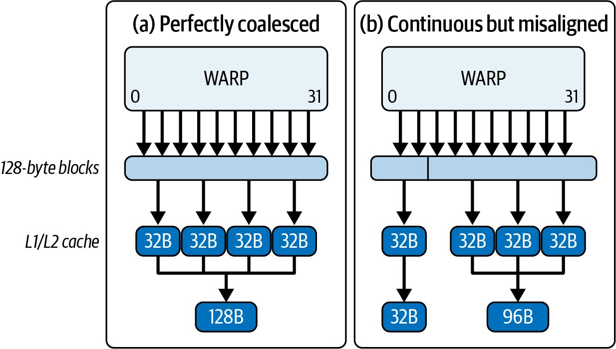
lines composed of four 32-byte sectors. This results in many more memory transac‐ tions retrieving unused data, which quickly eats up memory bandwidth. On a Blackwell GPU, per-device HBM3e bandwidth is up to 8 TB/s. Within the Grace Blackwell GB200 and GB300 (two GPU superchips), this increases 16 TB/s across both GPUs. Using uncoalesced memory accesses will leave most of this bandwidth unused due to excess memory transactions and stalls. In the uncoalesced case, each thread in a warp loads from scattered addresses. This results in many separate memory transactions. Even if threads in a warp access con‐ secutive addresses, if the first address isn’t 128-byte aligned, the warp’s request will span two 128-byte cache lines. For example, if a warp’s first thread starts at an address that isn’t 128-byte aligned, the warp’s memory request will cross a cache-line boundary, often resulting in two 128byte transactions instead of one. In that case the warp may fetch an extra sector beyond the optimal four sectors, for a total of five sectors across the two lines. This is a waste of bandwidth. Whether a misaligned, contiguous 128-byte warp load touches 5× 32 B sectors or 8× 32 B sectors depends on the start offset. Aligned accesses keep it to 4× 32 B sectors. In the coalesced case, however, threads load from consecutive addresses combined into a single wide transaction. Figure 7-1 compares coalesced and uncoalesced mem‐ ory access.
Figure 7-1. Comparing coalesced versus uncoalesced memory access pattern
In kernel code, this problem typically appears as strided or irregular indexing such that each thread reaches into different cache lines. When a kernel’s threads fetch data
240 | Chapter 7: Profiling and Tuning GPU Memory Access Patterns
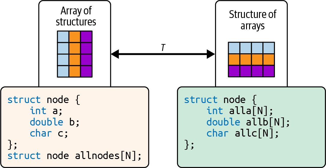
with strided or irregular indices, the GPU issues many small, uncoalesced global‐ memory transactions rather than a handful of full‐width loads. In Nsight Compute, the Memory Workload Analysis section will show lower Global Memory Load Efficiency, higher DRAM sector read counts, and average sectors per request above 4.0 when uncoalesced patterns are present. This is because more sec‐ tors are being fetched than a properly coalesced memory access pattern, and it indi‐ cates that you’re wasting bandwidth by fetching mostly unused bytes. And DRAM throughput percentage will remain well below peak. This confirms that your warp is spending cycles stalled on memory rather than driving the ALUs. To break out of this memory‐bound regime, you can reorganize your data so that each warp’s 32 threads load contiguous elements. Either index the array with input[idx] where idx = blockIdx.x * blockDim.x + threadIdx.x or switch to a structure‐of‐arrays (SoA) layout so that thread i always touches element i. The dif‐ ference between an array of structures (AoS) and an SoA is shown in Figure 7-2.
Figure 7-2. Array of structures (AoS) versus structure of arrays (SoA)
Once you make the change, the hardware will automatically combine the warp’s global memory loads into fewer, wider transactions with more usable (less wasted) data being returned. The Nsight Compute counters will immediately show improvement. Let’s demonstrate this with an example. The following before-and-after code demon‐ strates how restructuring global memory accesses from a strided pattern to a contigu‐ ous pattern produces a significant performance gain. Before example (C++): uncoalesced strided access. In this example, each thread copies from an input array with a stride of 2, causing misaligned memory accesses: #include <cuda_runtime.h> #include <iostream>
Coalesced Versus Uncoalesced Global Memory Access | 241
      __global__ void uncoalescedCopy(const float* __restrict__ in,
      float* __restrict__ out,
      int N, int stride) {
          // n = 1048576, stride = 2
          int idx = blockIdx.x * blockDim.x + threadIdx.x;
          if (idx < N) {
              // Loads from in[] with a stride, causing
              // multiple memory segments to be fetched
              out[idx] = in[idx * stride];
          }
      }
      int main() {
          const int N = 1 << 20;
          const int stride = 2;
           float* h_in = nullptr;
           float* h_out = nullptr;
           cudaMallocHost(&h_in, N * stride * sizeof(float));
           cudaMallocHost(&h_out, N * sizeof(float));
           for (int i = 0; i < N * stride; ++i) {
               h_in[i] = static_cast<float>(i);
           }
           float *d_in, *d_out;
           cudaMalloc(&d_in, N * stride * sizeof(float));
           cudaMalloc(&d_out, N * sizeof(float));
           cudaMemcpy(d_in, h_in, N * stride * sizeof(float),
             cudaMemcpyHostToDevice);
           // Number of threads per block (multiple of 32)
           const int threadsPerBlock = 256;
           // Number of blocks per grid
           const int blocksPerGrid = (N + threadsPerBlock - 1) /
             threadsPerBlock;
           uncoalescedCopy<<<blocksPerGrid,
             threadsPerBlock>>>(d_in, d_out, N, stride);
           cudaDeviceSynchronize();
           cudaFree(d_in);
           cudaFree(d_out);
           cudaFreeHost(h_in);
           cudaFreeHost(h_out);
           return 0;
      }
The CUDA C++ kernel issues global memory loads at addresses separated by a stride
> 1, which is, by definition, noncontiguous. This causes each warp to generate multi‐
ple small transactions instead of a single wide transaction.
242 | Chapter 7: Profiling and Tuning GPU Memory Access Patterns
Before example (PyTorch). In PyTorch, an analogous situation can be created using a strided index for a gather operation: import torch
    def uncoalesced_copy(input_tensor, stride):
        # Flatten to 1D so we know exactly
        #   which dimension we're indexing
        flat_tensor = input_tensor.contiguous().view(-1)
        # Generate indices with a fixed stride to gather
        assert flat_tensor.numel() % stride == 0,"stride must divide tensor length"
        idx = torch.arange(0, flat_tensor.numel(), stride,
            device=flat_tensor.device, dtype=torch.long)
        # index_select uses a gather kernel that issues uncoalesced loads
        return torch.index_select(flat_tensor, 0, idx)
    # Usage
    n, stride = 1 << 20, 2
    inp = torch.arange(n * stride, device='cuda',
                       dtype=torch.float32)
    out = uncoalesced_copy(inp, stride)
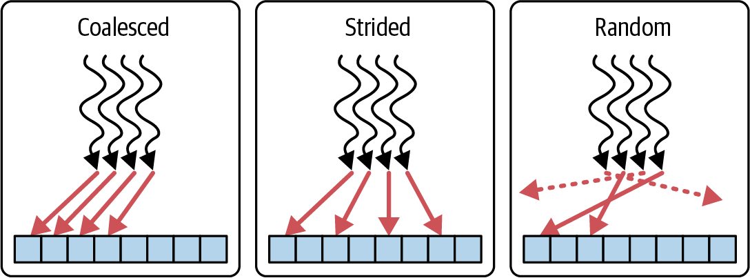
This PyTorch snippet uses torch.index_select with a strided index pattern, which causes the underlying GPU gather kernel to perform uncoalesced loads. Specifically, a warp of 32 threads will access addresses that are stride * 4 bytes apart. This does not allow a single wide transaction and instead generates 32 separate loads. Each thread loads a value from inp that is far apart in memory from the value loaded by the next thread, which prevents coalescing. Figure 7-3 shows the coalesced versus strided access pattern—as well as random access.
Figure 7-3. Coalesced, strided, and random memory access patterns
After running the C++ and PyTorch codes on a GPU, we measure performance met‐ rics. In the uncoalesced version, each warp’s memory request is broken into 8 sepa‐ rate 32-byte sectors on average. Since each 128-byte cache line fetch is split into 4 separate 32-byte sectors (more on this number 4 in a bit), the access pattern spans two lines per warp to retrieve the 8 separate 32-byte sectors.
Coalesced Versus Uncoalesced Global Memory Access | 243
In the unoptimized version, each warp’s uncoalesced loads break a single logical request into up to eight separate 32-byte sectors, ballooning transaction counts and starving the memory pipeline. As a result, Nsight Compute reports only about 25% of sustained peak dynamic random-access memory (DRAM) throughput. Now, let’s optimize this by coalescing the memory accesses and making threads read contiguous elements so each warp issues fewer, larger transactions. After example (C++): coalesced access. By simply removing the stride (or setting it to 1), each thread copies a contiguous element. This alignment of thread accesses allows the hardware to coalesce memory requests into full 128-byte transactions: #include <cuda_runtime.h> #include <iostream>
      __global__ void coalescedCopy(const float* __restrict__ in,
                                   float* __restrict__ out,
                                   int n) {
          int idx = blockIdx.x * blockDim.x + threadIdx.x;
          if (idx < n) {
              // Contiguous load
              // Threads copy neighboring elements
              out[idx] = in[idx];
          }
      }
      int main() {
          const int n = 1 << 20;
          const size_t bytes = n * sizeof(float);
           // 1) Allocate pinned host memory
           float *h_in = nullptr, *h_out = nullptr;
           cudaMallocHost(&h_in, bytes); // page-locked host alloc
           cudaMallocHost(&h_out, bytes);
           // 2) Initialize input
           for (int i = 0; i < n; ++i) {
               h_in[i] = static_cast<float>(i);
           }
           // 3) Allocate device memory
           float *d_in = nullptr, *d_out = nullptr;
           cudaMalloc(&d_in, bytes);
           cudaMalloc(&d_out, bytes);
           // 4) Copy to device
           cudaMemcpy(d_in, h_in, bytes,
             cudaMemcpyHostToDevice);
           // 5) Launch kernel
           dim3 block(256);
244 | Chapter 7: Profiling and Tuning GPU Memory Access Patterns
          dim3 grid((n + block.x - 1) / block.x);
          coalescedCopy<<<grid, block>>>(d_in, d_out, n);
          cudaDeviceSynchronize();
          // 6) Copy back to host
          cudaMemcpy(h_out, d_out, bytes,
            cudaMemcpyDeviceToHost);
          // 7) Clean up
          cudaFree(d_in);
          cudaFree(d_out);
          cudaFreeHost(h_in);
          cudaFreeHost(h_out);
return 0; } We leave out the coalesced PyTorch implementation for brevity since it’s already built into PyTorch. A coalesced version in PyTorch would simply do something like out = inp.clone(). This copies contiguous elements efficiently. In fact, clone() on a con‐ tiguous tensor uses a vectorized memory copy under the hood, analogous to our coa‐ lesced kernel.
                    You can also use torch.compile with the default TorchInductor
                    backend to reduce redundant copies and to fuse adjacent opera‐
                    tions when safe. clone() is already a device-to-device copy, so it’s
                    typically not fused into a separate custom kernel. Enable autotun‐
                    ing (e.g., mode="max-autotune") to help TorchInductor pick coa‐
                    lesced and vectorized schedules when shapes are stable. We’ll cover
                    the PyTorch compiler in depth in Chapters 13 and 14.
With coalesced access, or no stride, each warp’s threads access adjacent addresses. In this case, the hardware coalesces each warp’s loads into the minimum number of 128byte transactions—often one 128-byte transaction per warp when the first address is 128-byte aligned, or two if the access straddles a boundary. Table 7-1 shows the dra‐ matic improvements resulting from this optimization.
Table 7-1. Coalesced versus uncoalesced memory access performance Metric Before (uncoalesced) After (coalesced) DRAM throughput (% of peak) 25% 90% (3.6×) Global Memory Load Efficiency 23% 99% Average sectors per request 8.0 4.0 (optimal) SM Active % 62% 99% Kernel execution time (ms) 4.8 ms 1.3 ms (3.7×)
Coalesced Versus Uncoalesced Global Memory Access | 245
                    Note: The numeric values in all metrics tables are illustrative to
                    explain the concepts. For actual benchmark results on different
                    GPU architectures, see the GitHub repository.
After fixing the data layout and coalescing global memory accesses, DRAM through‐ put rises from 25% to 90% of peak, about 3.6× higher. Kernel execution time improves by about 3.7×, from 4.8 ms to 1.3 ms, as fewer stalls free the SMs to make forward progress. Global Memory Load Efficiency rises from 23% to 99%, meaning nearly every fetched byte is useful. At the same time, Average Sectors per Request falls to about 4.0.
                    A value near 4.0 means the warp’s loads are fully coalesced. With
                    the first address 128-byte aligned, all 32 threads map to one 128-
                    byte line. This line has four 32-byte sectors, so the metric reports
                    an average of 4.0 sectors per request.
In the worst case with strided or scattered access, the value can approach 32 because activity is reported in 32-byte sectors at L2. Values above 4.0 indicate uncoalesced or misaligned access. In an unoptimized version, uncoalesced loads can break a single logical access into many sectors per request, approaching the worst case. Here we are at about 4.0 sectors per request, which indicates that requests map cleanly to 128-byte lines with no unused sectors. With fewer memory stalls, SM Active percent improves from 62% to 99%. In summary, by aligning each warp’s threads on successive addresses, the GPU’s memory controller can service each warp with a few large transactions instead of dozens of tiny ones. This boosts the Global Memory Load Efficiency (fraction of each transaction that returns useful data) to near 100% and raises SM Active % by keeping warps busy instead of idle. And with that, you’ve seen how coalescing reshapes your thread-to-address mapping so an entire warp’s loads line up on the GPU’s 128-byte segments. However, even a fully coalesced warp still issues 32 individual 4-byte reads under the hood, one per thread, forcing the hardware to stitch them back together into each 128-byte transaction. To eliminate that last layer of inefficiency, we turn to vectorized memory access: hav‐ ing each thread fetch a wider, aligned chunk (e.g., a 16-byte float4) in a single instruction so that a coalesced warp issues exactly four 128-byte transactions, not 32. Let’s dive into how to pack your per-thread loads into CUDA’s built-in vector types.
246 | Chapter 7: Profiling and Tuning GPU Memory Access Patterns
Vectorized Memory Access While memory coalescing is a runtime hardware optimization on NVIDIA GPUs, vectorized memory access is a compile-time strategy in which each load or store instruction explicitly fetches multiple contiguous elements (e.g., float4, or 16 bytes) per thread. This reduces instruction count and eliminates stitching overhead. Efficient global‐memory access on Blackwell relies on matching your loads to the GPU’s native 128-byte transaction size. When each thread reads only a 4-byte float, a 32-thread warp still has to stitch together 32 4-byte requests to fill one 128-byte line. In ideal coalesced cases, a warp that reads 32 4-byte words aligned to a 128-byte boundary maps to exactly four 32-byte sectors. Nsight Compute captures this waste in the average sectors per request metric, which can climb well above 4.0 when your accesses are misaligned, strided, or scattered. As such, you’ll see Global Memory Load Efficiency drop as bandwidth goes underutilized. The fix is to bundle each thread’s work into a larger, naturally aligned vector that maps cleanly onto those 128-byte transactions. CUDA’s built-in float4 type does exactly that: it packs four 4-byte floats into a 16-byte struct guaranteed by the com‐ piler to be 16-byte aligned. For illustration purposes, it looks something like the fol‐ lowing code: // Example of a custom float4 for illustration purposes. // Note: it's recommended to use the built-in CUDA float4 type. // Note: if N is not divisible by 4, handle the last N % 4 elements // (e.g., a short scalar cleanup) or assert divisibility in host code. The // input and output pointers must be 16-byte aligned for float4 loads/stores. struct my_float4 { float x; // 4 bytes float y; // 4 bytes float z; // 4 bytes float w; // 4 bytes };
When all 32 threads in a warp issue a float4 load, they together fetch 32 × 16 bytes = 512 bytes of contiguous data, which the Blackwell memory controller then splits into exactly four 128-byte transactions (512 bytes ÷ 128 bytes per transaction = 4 transac‐ tions). This preserves the ideal 4.0 sectors per 128-byte transaction (discussed earlier re: coalesced memory access) because the warp requests 512 bytes, and the hardware services the request with four aligned 128-byte transactions for a total of 16 sectors, each fully utilized. Compared to an unaligned or strided case that can inflate sector counts, vectorized float4 loads reduce per-thread load instructions by 4×. This helps maintain the ideal 4.0 sectors per request when alignment is satisfied.
Vectorized Memory Access | 247
                    High-level GPU compilers like the PyTorch compiler can often
                    generate vectorized memory operations when alignment and conti‐
                    guity requirements are met. You can encourage this behavior by
                    using per-thread tiles that match vector widths. As such, frame‐
                    works can usually achieve a similar reduction in memory transac‐
                    tions under the hood. However, it’s still beneficial to align data
                    properly from the start.
As a result of this vectorized memory access optimization, global memory load effi‐ ciency increases toward 100%. Sectors per transaction remain at 4.0 when each 128byte transaction is fully utilized, while the warp issues multiple aligned transactions to serve a wider request. Vectorized loads reduce the number of memory instructions per byte moved and often increase effective bandwidth. To benefit from vectorized loads, data pointers must be aligned to the vector width. The CUDA runtime and driver allocation func‐ tions, such as cudaMalloc return device pointers aligned to at least 256 bytes. The base alignment is sufficient for 16-byte and 32-byte vector alignment at the allo‐ cation boundary. Adding an element offset can break alignment if the offset is not a multiple of the vector width. The following cast asserts the intended type to the com‐ piler and assumes the pointer is already correctly aligned: auto ptr4 = reinterpret_cast<const float4*>(ptr);
Make sure the pointer value is a multiple of 16 bytes (4 floats) before casting. This is because cudaMalloc() returns at least 256-byte alignment. Adding an element offset can break alignment if the offset is not a multiple of 4 floats. Correct alignment is a precondition for vectorized loads. With a base address aligned to 32 bytes, each thread reads 32 bytes per iteration, typi‐ cally compiling into two 16-byte vector load instructions per thread (Hopper) or one 32-byte load instruction (Blackwell). A 32-thread warp therefore requests 1,024 bytes. Each 128-byte cache line comprises four 32-byte sectors. As such, the warp generates eight aligned 128-byte transactions for a total of 32 sectors when accesses are aligned properly. This way, each access falls on a natural boundary and avoids split transactions. It’s worth noting that CUDA, as of this writing, does not provide a built-in 8-float aggregate CUDA vector type (e.g., eight combined float32s) in its <vector_ types.h>. You can define your own struct of 8 float values, then load it as two float4 values per thread. You would use 32-byte alignment on the type with alignas(32). This way, the pointer value is a multiple of 32 bytes. Global memory vector instructions on modern GPUs typically load 16 bytes per thread (Hopper) or 32 bytes per thread (Blackwell). In the case of Hopper’s 16 bytes per thread, an 8-float aggregate load will compile into two 16-byte loads per thread to include all 32 bytes.
248 | Chapter 7: Profiling and Tuning GPU Memory Access Patterns
Blackwell, on the other hand, would compile into a single 32-byte load per thread when using proper 32-byte aligned data. With 32-byte per-thread loads (e.g., 8 floats × 4 bytes per float), a warp moves 1,024 bytes (1,024 bytes = 32 threads per warp × 32 bytes per thread). This typically maps to 8 × 128-byte lines since each line consists of four 32-byte sectors. With 16-byte per-thread loads (e.g., four float4s), a warp moves 512 bytes (512 bytes = 32 threads per warp × 16 bytes per thread) or 4 × 128-byte lines. When the base pointer and perthread stride are naturally aligned, the hardware coalescer combines lane accesses into full lines and avoids split sectors. This type of mechanical sympathy is crucial to achieving peak throughput. Therefore, for 256-bit loads on Blackwell, you should enforce 32-byte alignment to maintain peak performance. Let’s see an example of scalar versus vectorized memory access in a simple vector copy kernel. Before example (C++): scalar copy. Each thread copies one float: #include <cuda_runtime.h>
    __global__ void copyScalar(
    const float* __restrict__ in,
    float* __restrict__ out, int N) {
        int idx = blockIdx.x * blockDim.x + threadIdx.x;
        if (idx < N) {
            // Scalar load: 4-byte copy per thread
            out[idx] = in[idx];
        }
    }
    int main() {
        const int N = 1 << 20;
        float* h_in = nullptr;
        float* h_out = nullptr;
        cudaMallocHost(&h_in, N * sizeof(float));
        cudaMallocHost(&h_out, N * sizeof(float));
for (int i = 0; i < N; ++i) h_in[i] = float(i);
        float *d_in, *d_out;
        cudaMalloc(&d_in, N * sizeof(float));
        cudaMalloc(&d_out, N * sizeof(float));
        cudaMemcpy(d_in, h_in, N * sizeof(float), cudaMemcpyHostToDevice);
        dim3 block(256), grid((N + 255) / 256);
        copyScalar<<<grid, block>>>(d_in, d_out, N);
        cudaDeviceSynchronize();
        cudaFree(d_in); cudaFree(d_out);
        cudaFreeHost(h_in);
Vectorized Memory Access | 249
          cudaFreeHost(h_out);
          return 0;
      }
Before example (PyTorch). A scalar elementwise copy in PyTorch could be done with a
Python loop for illustration:
      import torch
      def copy_scalar(inp: torch.Tensor) -> torch.Tensor:
          out = torch.empty_like(inp)
          flat_in = inp.view(-1)
          flat_out = out.view(-1)
          for i in range(flat_in.numel()):
              # Each iteration issues a 4-byte load on the GPU
              # This is extremely slow. DO NOT DO THIS!
              # Use vectorized operations to avoid Python loops
              # on GPU tensors as shown in optimized version
              flat_out[i] = flat_in[i]
          return out
      # Usage
      N = 1 << 20
      inp = torch.arange(N, device='cuda', dtype=torch.float32)
      out = copy_scalar(inp)
With scalar 4-byte loads, a warp often issues one 128-byte transaction for 128 bytes
when aligned. Otherwise, it uses two transactions if the access straddles a 128-byte
boundary. Using float4 (16 bytes per thread) means each warp issues 4× more data
per memory instruction—512 bytes per warp—split into four 128-byte transactions.
This allows the transfer to complete in fewer instructions. Next, let’s optimize by
using vector loads.
After example (C++): vectorized copy. Each thread copies a float4 (16 bytes):
      #include <cuda_runtime.h>
      // 16-byte (128-bit) vector copy: one float4 per thread
      static_assert(alignof(float4) == 16, "float4 alignment must be 16 bytes");
      __global__ void copyVector16B(const float4* __restrict__ in,
                                    float4* __restrict__ out,
                                    int N4) // number of float4 elements
      {
          int idx = blockIdx.x * blockDim.x + threadIdx.x;
          if (idx < N4) {
              // Per-thread 16B load+store.
              // On sm_90, NVCC emits ld.global.v4.f32 / st.global.v4.f32.
              // for 16-byte vector loads and stores
              // On sm_90 (Hopper) (Blackwell), NVCC emits
              // ld.global.v8.f32 and st.global.v8.f32 for 32-byte aligned data
              out[idx] = in[idx];
          }
250 | Chapter 7: Profiling and Tuning GPU Memory Access Patterns
}
    int main() {
        const int N = 1 << 20;     // total number of floats
        const int N4 = N / 4;      // total number of float4s (16B chunks)
        float4 *d_in = nullptr, *d_out = nullptr;
        cudaMalloc(&d_in, N4 * sizeof(float4));      // >=256B aligned
        cudaMalloc(&d_out, N4 * sizeof(float4));
        dim3 block(256);
        dim3 grid((N4 + block.x - 1) / block.x);
        copyVector16B<<<grid, block>>>(d_in, d_out, N4);
        cudaDeviceSynchronize();
        cudaFree(d_in);
        cudaFree(d_out);
        return 0;
    }
Here we use CUDA’s built-in float4 type from <cuda_runtime.h>. We launch N/4 threads to maintain 16-byte alignment and issue true vector loads/stores, and each thread copies one float4 (16 bytes). This means each thread handles four floats, and each warp handles 128 floats total in four transactions. cudaMalloc returns pointers aligned to at least 256 bytes which satisfies the float4 (16-byte) requirement and helps with 32-byte aligned vectors when you use 32-byte alignment for the data’s starting address. It’s important to note that misaligned casts can forfeit vectorization. Following is an example that takes advantage of Blackwell’s support for 32-byte vec‐ torized loads: // --- Blackwell-only variant: 32-byte per-thread vector copy // (PTX: ld.global.v8.f32) // Requires 32B alignment. #include <cuda_runtime.h>
    // Proof of 32-byte alignment
    static_assert(alignof(float8) == 32, "float8 alignment must be 32 bytes");
    struct alignas(32) float8 { float v[8]; };
    __global__ void copyVector32B(const float8* __restrict__ in,
                                  float8* __restrict__ out, int N8) {
        int idx = blockIdx.x * blockDim.x + threadIdx.x;
        if (idx < N8) {
            // Per-thread 32B load+store
            // NVCC emits ld.global.v8.f32/st.global.v8.f32 on sm_100
            out[idx] = in[idx];
        }
    }
    int main() {
        const int N = 1 << 20;
Vectorized Memory Access | 251
const int N8 = N / 8;
           float8 *d_in, *d_out;
           // cudaMalloc returns pointers aligned to ≥256 bytes
           // This will allow the compiler to emit
           // optimized ld.global.v8.f32 and st.global.v8.f32 instructions
           cudaMalloc(&d_in, N8 * sizeof(float8));
           cudaMalloc(&d_out, N8 * sizeof(float8));
           dim3 block(256), grid((N8 + block.x - 1) / block.x);
           copyVector32B<<<grid, block>>>(d_in, d_out, N8);
           cudaDeviceSynchronize();
           cudaFree(d_in); cudaFree(d_out);
           return 0;
      }
After example (PyTorch). We can simulate vectorized copy by using a tensor view and
clone:
      import torch
      def copy_vectorized(inp: torch.Tensor) -> torch.Tensor:
          # Reshape into groups of 4 floats for bulk copy
          vec = inp.view(-1, 4)
          # clone() on a contiguous CUDA tensor performs a device-to-device copy
          # using optimized runtime paths such as cudaMemcpyAsync().
           out_vec = vec.clone()
           return out_vec.view(-1)
      # Usage
      N = 1 << 20
      inp = torch.arange(N, device='cuda', dtype=torch.float32)
      out = copy_vectorized(inp)
Calling clone() on the reshaped tensor causes PyTorch to perform contiguous copies. This is in contrast to copying element by element. By using float4 vector loads, each thread moves 16 bytes per instruction, which is optimized for Hopper. (Blackwell supports 32-byte vector loads per thread.) A warp issues 512 bytes for that load, typically split into four 128-byte transactions when aligned. The benefit comes from fewer instructions per byte moved, better sector utilization, and proper align‐ ment to maximize memory throughput on modern GPUs. This shows far better uti‐ lization of memory bandwidth, as shown in Table 7-2.
252 | Chapter 7: Profiling and Tuning GPU Memory Access Patterns
                    Blackwell doubles the number of bytes for vector loads/stores per
                    thread relative to Hopper. With CUDA 13, Blackwell can perform
                    32-byte vector loads and stores instead of 16 bytes on Hopper. This
                    requires that the compiler can prove 32-byte alignment. Otherwise,
                    it may split the per-thread load/store into two 16-byte instructions.
                    This will increase the number of instructions required to load/store
                    the same amount of data which will negatively impact
                    performance.
By using properly aligned float4 vector loads, each thread moves 16 bytes per instruction. This shows far better utilization of memory bandwidth, as shown in the results in Table 7-2.
Table 7-2. Nsight Compute metrics for scalar versus vectorizing memory access Metric Before (scalar) After (vectorized) Global Memory Load Efficiency 28% 97% Average sectors per request 31.8 4.0 DRAM throughput (% of peak) 25% 90% (3.6×) Kernel execution time 4.2 ms 1.2 ms (3.5× improvement)
These metrics confirm the improvement. Global Memory Load Efficiency jumped from 28% to 97% (~3.5×), and percentage of peak DRAM throughput increased from 25% to 90% (~3.6×), trimming the overall kernel runtime by ~3.5×. This optimization trimmed the kernel execution runtime by roughly 3.5× from 4.2 ms down to 1.2 ms. Global Memory Load Efficiency jumps from 28% (scalar) to 97% (vectorized), meaning that almost every fetched 128-byte transaction is now used. The average sectors per request drops toward the 4.0 sector-per-line ideal value. This indicates that each 128-byte line is fully utilized. Each warp-wide float4 instruction issues four aligned 128-byte transactions to move 512 bytes. As such, every transac‐ tion is fully utilized. The reduction in memory requests and the replacement of four scalar loads with one vector load increase global memory load efficiency from 28% to 97% and raise sus‐ tained DRAM throughput from about 25% to about 90% of peak. In this case, warps are doing far fewer memory operations and get more data with each operation, so they spend much less time waiting on memory and more time executing useful work. The end result is a significantly faster kernel.
                    Vectorization reduces instruction count. Coalescing and alignment
                    improve the number of sectors per request.
Vectorized Memory Access | 253
Let’s quickly compare coalesced global memory access from the previous section to vectorized memory access discussed here. Coalescing makes sure threads in a warp all hit one big contiguous block. Vectorizing makes sure each thread fetches a wide chunk that exactly maps onto those big blocks. The differences are summarized in Table 7-3.
Table 7-3. Comparing coalesced memory access (previous section) and vectorized memory access Aspect Coalesced warp load (interthread) Vectorizing (intrathread) Granularity Threads ↔ contiguous memory addresses Per thread ↔ vector loads Typical fix Contiguous indexing (stride = 1) Use float4, a custom 32-byte struct with explicit 32-byte alignment, or a 32-byte-aligned vector type (e.g., Blackwell and CUDA 13+) Transactions/warp 32 threads × 4 bytes → 128 bytes, equal 32 threads × 16 bytes → 512 bytes, equal to 4 128-byte to 4 32-byte sectors if aligned (4 sectors) transactions, which correspond to 16 32-byte sectors (16 sectors) Instruction count Same number of loads 1 vector load instead of 4 scalars change Benefit Fewer scattered sectors Perfectly sized, fewer sectors
By combining both strategies, you ensure that warps hit contiguous blocks such that each thread fetches a wide, aligned vector. This helps you push your kernel’s memory bandwidth utilization to its peak and unlock the full power of your GPU. It’s worth noting that, prior to Blackwell and CUDA 13, global memory vector loads were limited to 16 bytes (128 bits) per thread. However, Blackwell and CUDA 13 added 32-byte (256-bit) load/store instructions and data types for specific vector types with 32-byte alignment. When available, prefer these wider 32-byte types and instructions for user-defined 8float aggregates. This will reduce the number of instructions needed to load and store wider 32-byte aligned data. Custom 8-float aggregates will still compile into two 16-byte loads unless you explic‐ itly use the 32-byte-aligned types that map to a single 32-byte instruction.
                     Even though a Blackwell thread can load a full 32-byte vector type,
                     the memory coalescer can still only service requests in 128-byte
                     chunks, or four 32-byte sectors. On Blackwell, a 32-thread warp
                     moving 32 B per thread transfers 1024 B (8 × 128 B lines). Hopper’s
                     16 B/thread variant moves 512 B (4 × 128 B). Note that the transac‐
                     tion count scales with bytes moved. Both are fully efficient when
                     properly aligned: 16-byte (Hopper) or 32-byte (Blackwell and
                     beyond).
254 | Chapter 7: Profiling and Tuning GPU Memory Access Patterns
Tiling and Data Reuse Using Shared Memory A common performance pitfall is repeatedly reading the same data from global mem‐ ory. Tiling is a technique to avoid this by loading chunks of data into faster on-chip shared memory—and reusing those chunks across many threads. For example, a naive matrix multiplication of size N × N might load each element of matrix A from HBM N times, once for each row of B it multiplies with. This results in N–1 redundant loads per element. And on Blackwell, which can easily execute tens of teraFLOPS (TFLOPS), redundant loads can waste memory bandwidth, which could otherwise be feeding more math operations to the GPU SMs. Tiling eliminates this waste by having each thread block pull a small submatrix (a tile) of A and B into shared memory exactly once. It then reuses the cached values across all threads for multiple multiply-accumulate operations. In our next example, we’ll use a 32 × 32 tile, which is a common choice that fits well in shared memory. Threads within a block can cooperatively load the tile into shared memory, then call __syncthreads() to synchronize the data. Then the threads perform parallel matrixmultiply computations using the data in shared memory. This amortizes the global memory access cost over many threads and computations. It’s worth noting that these tile loads are also arranged to be coalesced. Specifically, each warp loads a full 128byte segment from global memory into shared memory—consistent with the coalesc‐ ing example from earlier. By reading each element from DRAM only once (into shared memory) and reusing it for many calculations, we reduce global memory traffic. Let’s illustrate this with an N × N matrix multiplication example. First, consider a naive implementation. Before example (CUDA C++): naive matrix multiply. Each thread computes one ele‐ ment of the result matrix C, reading entire rows of A and columns of B from global memory for each output: #include <cuda_runtime.h> #include <iostream>
    __global__ void naiveMatMul(const float* A, const float* B, float* C, int N) {
        int row = blockIdx.y * blockDim.y + threadIdx.y;
        int col = blockIdx.x * blockDim.x + threadIdx.x;
        if (row < N && col < N) {
            float sum = 0.0f;
            for (int k = 0; k < N; ++k) {
                // Each thread loads A[row, k] and B[k, col]
                // from global memory for every k.
                // This is very memory heavy.
                sum += A[row * N + k] * B[k * N + col];
            }
            C[row * N + col] = sum;
Tiling and Data Reuse Using Shared Memory | 255
           }
      }
      int main() {
          const int N = 1024;
          size_t bytes = N * N * sizeof(float);
           float* h_A = nullptr;
           float* h_B = nullptr;
           float* h_C = nullptr;
           cudaMallocHost(&h_A, N*N * sizeof(float));
           cudaMallocHost(&h_B, N*N * sizeof(float));
           cudaMallocHost(&h_C, N*N * sizeof(float));
for (int i = 0; i < N*N; ++i) { h_A[i] = 1.0f; h_B[i] = 1.0f; }
           float *d_A, *d_B, *d_C;
           cudaMalloc(&d_A, bytes);
           cudaMalloc(&d_B, bytes);
           cudaMalloc(&d_C, bytes);
           cudaMemcpy(d_A, h_A, bytes, cudaMemcpyHostToDevice);
           cudaMemcpy(d_B, h_B, bytes, cudaMemcpyHostToDevice);
           dim3 block(32, 32);
           dim3 grid((N + 31) / 32, (N + 31) / 32);
           naiveMatMul<<<grid, block>>>(d_A, d_B, d_C, N);
           cudaDeviceSynchronize();
           cudaFree(d_A);
           cudaFree(d_B);
           cudaFree(d_C);
           cudaFreeHost(h_A);
           cudaFreeHost(h_B);
           cudaFreeHost(h_C);
           return 0;
      }
This CUDA C++ kernel issues global memory loads for every multiplication inside
the inner loop. Each thread reads A[row, k] and B[k, col] from DRAM for every k,
causing massive redundant traffic. The result is a heavily memory-bound kernel with
low SM utilization and frequent stalls waiting on global memory. Here is the PyTorch
version of the naive matrix multiplication:
      import torch
      def naive_matmul(A, B):
          N = A.size(0)
          C = torch.zeros((N, N), device='cuda')
          for i in range(N):
              for j in range(N):
                  # Each dot product loads A[i,:] B[:,j] from global memory repeatedly
                  C[i, j] = (A[i, :] * B[:, j]).sum()
          return C
256 | Chapter 7: Profiling and Tuning GPU Memory Access Patterns
    # Usage
    N = 1024
    A = torch.ones((N, N), device='cuda', dtype=torch.float32)
    B = torch.ones((N, N), device='cuda', dtype=torch.float32)
    C = naive_matmul(A, B)
This PyTorch implementation uses nested Python loops. While the innermost opera‐
tions are offloaded to GPU as elementwise multiply and sum operations, it still trig‐
gers repeated global memory loads under the hood for each dot product. This mimics
the memory-bound behavior of the naive CUDA kernel since the GPU spends most
cycles waiting on memory rather than computing multiplications.
                This PyTorch code is extremely slow on purpose to illustrate the
                extreme case of performing redundant global memory access loads
                inside of a loop. In practice, frameworks like PyTorch use opti‐
                mized kernels for this type of operation.
Now, let’s apply tiling to improve this. We divide the matrices into 32 × 32 tiles. 32 × 32 is a convenient tile size since it aligns with a warp size of 32, it fits well in shared memory, and it maps to a full warp of 32 threads reading each row. This allows each warp to collaboratively load and process one single row (per tile) at a time. As such, each thread block loads one 32 × 32 tile of A and one 32 × 32 tile of B into shared memory, performs the 32 × 32 matrix multiplies, and accumulates the results. This way, each element of A and B is loaded from HBM only once per tile instead of 32 times in the naive version. The optimized version using shared memory to cache tiles for matrix multiplies is shown here: #include <cuda_runtime.h> #include <iostream> #define TILE_SIZE 32
    __global__ void tiledMatMul(const float* A, const float* B, float* C, int N) {
        __shared__ float sA[TILE_SIZE][TILE_SIZE];
        __shared__ float sB[TILE_SIZE][TILE_SIZE];
        int row = blockIdx.y * TILE_SIZE + threadIdx.y;
        int col = blockIdx.x * TILE_SIZE + threadIdx.x;
        float sum = 0.0f;
        // compute partial results using the tile
        // in shared memory
        for (int t = 0; t < N; t += TILE_SIZE) {
            // Cooperative load of a tile of A and B into shared memory
            // Load tile A with boundary check
            if (row < N && (t + threadIdx.x) < N) {
                sA[threadIdx.y][threadIdx.x] = A[row * N + t + threadIdx.x];
            } else {
Tiling and Data Reuse Using Shared Memory | 257
                      sA[threadIdx.y][threadIdx.x] = 0.0f;
                }
                // Load tile B with boundary check
                if ((t + threadIdx.y) < N && col < N) {
                    sB[threadIdx.y][threadIdx.x] = B[(t + threadIdx.y) * N + col];
                } else {
                    sB[threadIdx.y][threadIdx.x] = 0.0f;
                }
                // We will optimize this later to use a
                // thread-block-scoped cooperative-groups barrier
                __syncthreads();
                // Compute using the tile loaded in shared memory
                for (int k = 0; k < TILE_SIZE; ++k) {
                    sum += sA[threadIdx.y][k] * sB[k][threadIdx.x];
                }
                // We will optimize this later to use a
                // thread-block-scoped cooperative-groups barrier
                __syncthreads();
           }
           if (row < N && col < N) {
               C[row * N + col] = sum;
           }
      }
      int main() {
          const int N = 1024;
          size_t bytes = N * N * sizeof(float);
           float* h_A = nullptr;
           float* h_B = nullptr;
           float* h_C = nullptr;
           cudaMallocHost(&h_A, N*N * sizeof(float));
           cudaMallocHost(&h_B, N*N * sizeof(float));
           cudaMallocHost(&h_C, N*N * sizeof(float));
for (int i = 0; i < N*N; ++i) { h_A[i] = 1.0f; h_B[i] = 1.0f; }
           float *d_A, *d_B, *d_C;
           cudaMalloc(&d_A, bytes);
           cudaMalloc(&d_B, bytes);
           cudaMalloc(&d_C, bytes);
           cudaMemcpy(d_A, h_A, bytes, cudaMemcpyHostToDevice);
           cudaMemcpy(d_B, h_B, bytes, cudaMemcpyHostToDevice);
           dim3 block(TILE_SIZE, TILE_SIZE);
           dim3 grid((N + TILE_SIZE - 1) / TILE_SIZE, (N + TILE_SIZE - 1) / TILE_SIZE);
           tiledMatMul<<<grid, block>>>(d_A, d_B, d_C, N);
258 | Chapter 7: Profiling and Tuning GPU Memory Access Patterns
        // synchronize the kernel with the device
        // for timing accuracy
        cudaDeviceSynchronize();
        cudaFree(d_A);
        cudaFree(d_B);
        cudaFree(d_C);
        cudaFreeHost(h_A);
        cudaFreeHost(h_B);
        cudaFreeHost(h_C);
        return 0;
    }
In this tiled kernel, each block cooperatively loads a 32 × 32 tile of A (into sA) and a 32 × 32 tile of B (into sB) from global memory. These loads happen in the first two lines inside the loop and are followed by __syncthreads() to ensure the tile is fully loaded before use. Then the block performs 32 × 32 multiply-accumulate operations using the shared memory tiles. This inner loop, running over k in steps of 32, reuses each loaded value 32×, yielding a 32× reduction in global memory reads for those elements. After finishing all tile iterations, each thread writes its result to C. The result is a dra‐ matic 8× reduction in global memory accesses per thread, as you’ll see in a bit.
                These examples are focused on memory access patterns and are
                using FP32 CUDA cores—not the reduced-precision Tensor Cores.
                Chapter 9 demonstrates the use of reduced-precision computations
                (e.g., 16-bit, 8-bit, 4-bit) to improve performance even further.
This PyTorch version manually tiles the matrices and invokes torch.mm on each tile. PyTorch’s torch.mm leverages NVIDIA’s cuBLAS and CUTLASS, which implement shared memory tiling and reuse internally at the C++ level. Here is the PyTorch ver‐ sion of the tiled matrix multiply: import torch
    def tiled_matmul(A, B, tile_size=32):
        N = A.size(0)
        C = torch.zeros((N, N), device='cuda')
        for i in range(0, N, tile_size):
            for j in range(0, N, tile_size):
                C_block = torch.zeros((tile_size, tile_size), device='cuda')
                for k in range(0, N, tile_size):
                    A_block = A[i:i+tile_size, k:k+tile_size]
                    B_block = B[k:k+tile_size, j:j+tile_size]
                    # torch.mm uses an optimized kernel (likely tiling internally)
                    C_block += torch.mm(A_block, B_block)
                C[i:i+tile_size, j:j+tile_size] = C_block
Tiling and Data Reuse Using Shared Memory | 259
return C
      # Usage
      N = 1024
      A = torch.ones((N, N), device='cuda', dtype=torch.float32)
      B = torch.ones((N, N), device='cuda', dtype=torch.float32)
      C = tiled_matmul(A, B)
                    With a 32 × 32 tile, threads in a warp will contend for the same
                    shared-memory bank when they all access the same column. In
                    practice, you can avoid this by padding the tile to 33 columns—or
                    using techniques like swizzling—so that each access falls in a differ‐
                    ent bank. We will apply this optimization in the next section. For
                    now, let’s focus on tiling as an optimization on its own.
The performance impact of tiling is significant. By structuring the computation in tiles and reusing data in shared memory, we reduce DRAM traffic and raise arith‐ metic intensity because each byte retrieved from memory is used for many more floating-point operations. Along with fewer global memory transactions, we also observe higher achieved occupancy. Table 7-4 compares key metrics before and after applying shared memory tiling.
Table 7-4. Performance improvement with shared memory tiling Metric Before After Notes (naive kernel) (tiled kernel) DRAM throughput 90% 25% (3.6× less) Naive uses more bandwidth, but it’s wasteful. The tile (% of peak) implementation is lower because it’s more efficient after tiling due to fewer redundant loads. Achieved occupancy 42% 89% More resident warps make forward progress with fewer stalls. (%) Floating-point 15 GFLOPS 170 GFLOPS Small matrix size limits the absolute value. Reuse increases throughput sustained compute. (GFLOPS) (The absolute GFLOPS numbers are low because the matrix size (N = 1,024) is small and the kernel is memory limited.) Global memory 9800 1200 Each element is fetched once per tile instead of 32 times (once load sectors per thread). Total number of 32-byte sector reads issued by the kernel. The decrease reflects the elimination of redundant loads thanks to shared-memory tiling. Shared memory 52% 99% Tiled kernel access pattern avoids memory-bank conflicts on sA throughput (% of and sB. peak)
260 | Chapter 7: Profiling and Tuning GPU Memory Access Patterns
Staging 32 × 32 tiles in shared memory makes sure that each element is fetched once from DRAM and reused across all threads in a block. DRAM throughput falls from 90% to 25%, a reduction of about 3.6×, which is expected when redundant traffic is removed. The drop in DRAM throughput is desirable because the kernel now performs more work per byte moved. Arithmetic intensity increases, and sustained floating-point throughput rises from 15 GFLOPS to 170 GFLOPS, a gain of nearly 11×.
               The optimized 170 GFLOPS is far below Blackwell’s theoretical
               FP32 peak near 80 TFLOPS. This is expected for small tiles and fre‐
               quent memory access. The important result is the 11× improve‐
               ment after removing the memory bottleneck. Larger problems or
               more compute work per byte would move performance closer to
               peak.
This shift in arithmetic intensity moves the kernel from memory bound toward com‐ pute bound, which is ideal because performance becomes limited by abundant floating-point throughput rather than comparatively scarce chip bandwidth. Global memory load sectors drop substantially from 9,800 down to 1,200 because each ele‐ ment is fetched once into shared memory and reused across threads. This eliminates redundant loads. The tiled kernel also accesses sA and sB in a way that avoids sharedmemory bank conflicts, which is why shared memory throughput approaches 100%. Overall, we shifted this kernel from memory bound to compute bound, which was the goal. We successfully relieved memory pressure, freed up the memory bus for other useful work, and achieved higher compute throughput. We also see a large increase in achieved occupancy percentage from 42% to 89%. This metric nearly doubles because the tiled kernel keeps allowing more resident warps to make progress with fewer stalls. As such, the SMs remain busy more consistently. By introducing shared memory tiling, we increased per-thread work without increas‐ ing per-thread resource usage beyond available registers and shared memory. This helped our kernel achieve higher occupancy and utilization, which is important on GPUs like Blackwell, which offer a very large register file (65,536 32-bit registers per SM) that threads can exploit up to the 255-register per-thread limit without spilling.
               Recall that each thread can use up to 255 registers. Our tiling ker‐
               nel implementation stays within this limit, avoids register spilling,
               and preserves high performance.
Tiling and Data Reuse Using Shared Memory | 261
We can compare the arithmetic intensity of the naive and tiled kernels by examining their sustained FLOP rates and average DRAM bandwidth. The naive version ran at 15 GFLOPS while moving 10 GB/s of data on average, or 1.5 FLOPS per byte. The tiled implementation, by contrast, sustained 170 GFLOPS while moving 21 GB/s on average, or 8 FLOPS/byte. It might be tempting to increase the tile size further to 64 × 64 or 128 × 128 in order to reduce memory traffic even more and increase data reuse. Just remember that larger tiles consume more on-chip resources, including both registers and shared memory. This leaves less capacity for additional thread blocks on each SM. For instance, Blackwell GPUs provide up to 228 KB of allocatable shared memory per SM. This can easily accommodate a 64 × 64 tile of 4-byte floats in which each A and B tile requires 16 KB (16,384 bytes = 64 × 64 floats × 4 bytes per float). However, in addition to shared-memory usage, you need to budget for the additional registers per thread. Each Blackwell SM provides up to 64K registers (32-bit each) in total with a perthread maximum of 255 registers. When you launch a 32 × 32 thread block (1,024 threads) to compute a 64 × 64 tile, each thread handles a 2 × 2 subtile, which pro‐ duces 4 outputs. For a 64 × 64 tile size, you need the following: four accumulator registers (one per output), two registers for A-tile elements (reused across two outputs), two registers for B-tile elements (same reuse), and ~4 registers for loop counters, thread indices, and address arithmetic. In total, this is ~12 registers per thread. 12 registers per thread × 1,024 threads per block = 12,288 registers needed per thread block. And since each Blackwell SM has 65,536 32-bit registers (maximum 255 regis‐ ters per thread), in theory, up to 5 blocks’ worth of registers can fit (≈61,440 regis‐ ters). However, the SM can support only 2,048 concurrent threads (64 warps). So, in practice, occupancy is limited by the smaller limits of registers, shared memory, warps, and threads. For this configuration, two blocks per SM will saturate the 2,048thread limit.
                    If your kernel uses additional registers for double-buffering regis‐
                    ters, vectorized loads, etc., you can recalculate the occupancy
                    with cudaOccupancyMaxPotentialBlockSize or Nsight Compute’s
                    occupancy report.
For a 64 × 64 tile size, 22 registers per thread are needed for a total of 22,528 registers for a 32 × 32 thread block (1,024 threads). In this case, you can only fit up to two thread blocks per Blackwell SM. This translates to a maximum occupancy of only 2,048 threads—hitting the SM’s thread limit with only two blocks (out of the 16 maxi‐ mum concurrent blocks per SM).
262 | Chapter 7: Profiling and Tuning GPU Memory Access Patterns
A reduction in concurrent thread blocks caused by using a larger tile size will lower occupancy and hurt performance if you exceed the hardware’s limits. In practice, your tile dimensions must fit within the GPU’s shared-memory and register budgets to maintain high occupancy and throughput. For a Blackwell GPU with ~228 KB of allocatable shared memory per SM, a 64 × 64 tile (~16 KB per input matrix tile) might still fit, but doubling the tile dimensions squares the reuse factor while quadrupling shared memory usage. There are dimin‐ ishing returns and possible trade-offs. It is recommended to experiment with different tile dimensions to balance on-chip reuse against resource limits. A 32 × 32 tile is a solid starting point on modern NVI‐ DIA GPUs, but depending on your shared-memory and register usage, you may find that a slightly smaller or larger tile delivers better throughput.
               Libraries like CUTLASS also include profilers that automate this
               exploration, letting you find the optimal tile size for your kernel
               and hardware.
In short, we transformed a naive, global-memory-only matrix multiplication into a tiled implementation that uses shared memory. This enabled cooperative data reuse, reduced the number of DRAM transactions, and boosted arithmetic intensity. Both the CUDA C++ and PyTorch implementations benefited from this tiling technique. It’s worth noting that the tiling techniques we applied manually are exactly what highperformance GPU libraries do under the hood. NVIDIA’s CUTLASS library, for instance, provides templated components to implement general matrix multiplies (GEMMs) with multiple layers of tiling. These CUTLASS components load fragments of matrices into registers and shared memory—and then compute partial results much like our previous 32 × 32 tile example. In fact, NVIDIA’s optimized cuBLAS and cuDNN libraries use similar blocking strategies at the thread, warp, and block levels to achieve near-peak throughput. NVI‐ DIA even announced a Python-first API in early 2025 called cuTile that lets program‐ mers describe these tile shapes in a more convenient Pythonic way. In fact, NVIDIA has developed a Tile-based intermediate representation (IR) called TileIR to support cuTile and facilitate automatic compilation and tuning. Other high-performance libraries encapsulate these tiling patterns as well. For instance, NVIDIA’s CUTLASS C++ and Python libraries expose templated tile itera‐ tors and profilers. And PyTorch-based compilers like TorchInductor (using the OpenAI Triton library) generate tiled kernels automatically when shapes and align‐ ment permit. These libraries lower the barrier to using these tiling optimizations— and reduce the amount of boilerplate code.
Tiling and Data Reuse Using Shared Memory | 263
The key idea is that reusing data in registers/shared memory as much as possible before going back to DRAM is fundamental, and libraries encapsulate this. So when‐ ever possible, leverage these highly optimized libraries (or refer to them) for perform‐ ant tiling patterns. For instance, if you use torch.mm in PyTorch or cublasSgemm in your code, under the covers it’s doing exactly this kind of tiling and memory coalescing. This is why our PyTorch example saw the same benefits automatically. In practice, you would use high-performance libraries like cuBLAS and PyTorch’s torch.matmul, which already implement tiling and other optimizations in C++. In production code, directly using torch.mm or torch.matmul would produce the same benefits—and possibly more, thanks to highly tuned kernels.
                    While you can definitely reuse existing tiling libraries and frame‐
                    works, understanding how they work, as we’ve done here, is invalu‐
                    able for when you need to diagnose performance issues and
                    possibly write your own custom kernels for specialized situations
                    that these libraries and frameworks don’t cover. Just don’t forget to
                    give back to the community as they’ve given you a lot!
As mentioned earlier in this section, when using a 32 × 32 tile, the threads in a warp will contend for the same shared-memory bank when they access the same column. Let’s explain this issue—as well as some optimizations—in the next section.
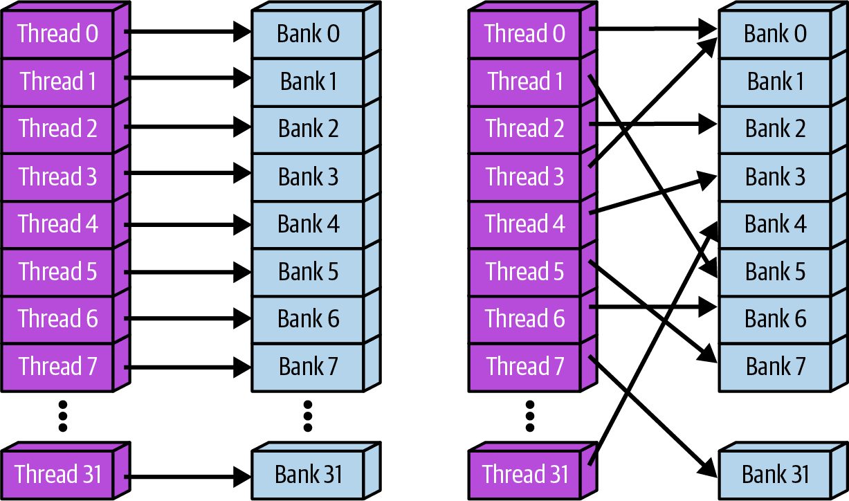
Avoid Shared-Memory Bank Conflicts On modern NVIDIA GPUs, including Blackwell, shared memory has 32 banks with a 4-byte bank width (i.e., addresses map mod 32 ). As such, a warp that strides by 128 B (32 floats × 4 B) maps all threads to the same bank. If multiple threads in a warp access the same bank, a bank conflict occurs. This forces the memory accesses to seri‐ alize, which negates the speed advantage of shared memory. In code, bank conflicts often occur when threads access a shared-memory array with a stride that causes them to fall into the same bank. Figure 7-4 shows two examples of conflict-free memory bank accesses.
264 | Chapter 7: Profiling and Tuning GPU Memory Access Patterns
Figure 7-4. No bank conflicts
Here, there are no two threads accessing the same memory bank concurrently. This is ideal. Figure 7-5 shows examples of both a 2-way and 16-way bank conflict.
Figure 7-5. 2-way and 16-way bank conflicts
Here, multiple threads are accessing the same memory bank, which will cause con‐ flicts and impact performance. A classic example of a bank conflict is a naive matrix transpose that uses a 32 × 32 shared memory tile. If 32 threads each read tile[i] [threadIdx.x] such that the same column index (threadIdx.x) is read across
Avoid Shared-Memory Bank Conflicts | 265
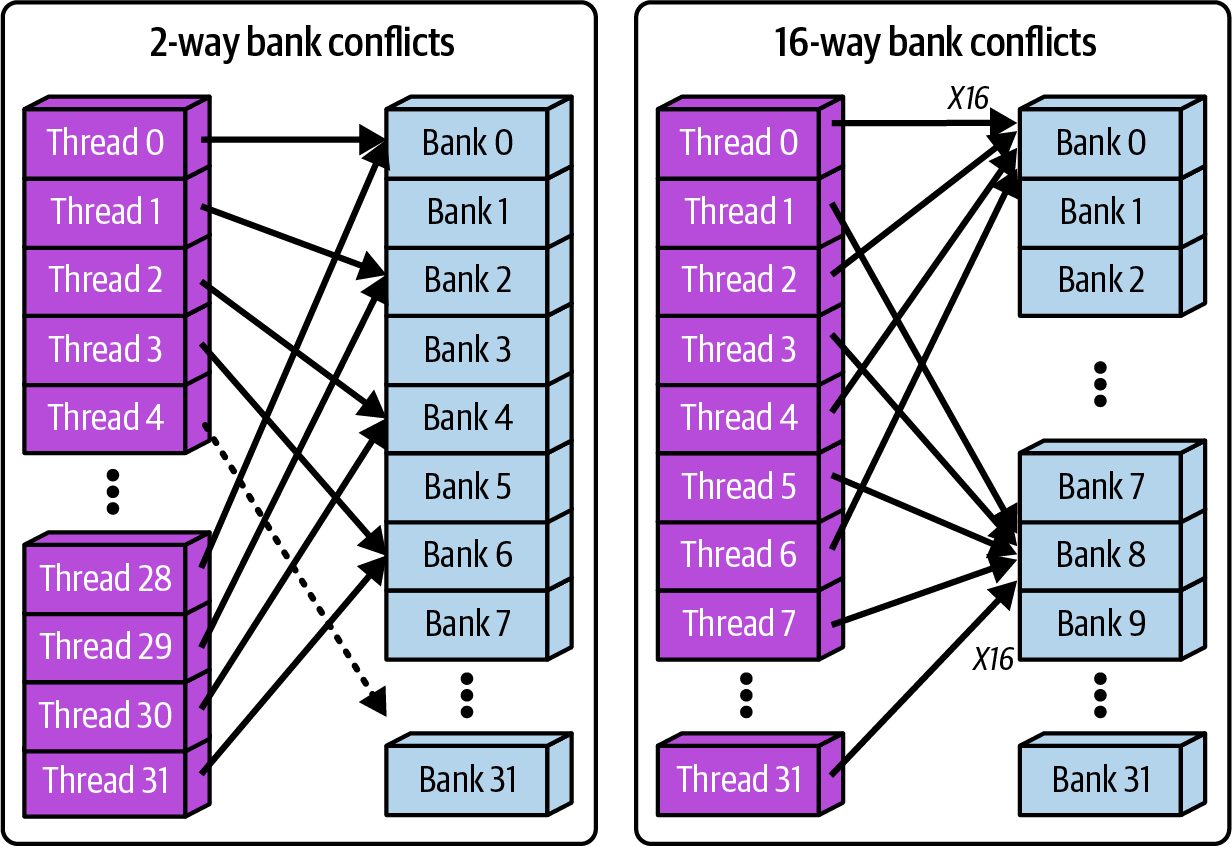
different rows (i), all 32 threads in the warp will each access memory addresses that lie in the same shared-memory bank, causing a 32-way bank conflict. Specifically, during a matrix transpose, you are reading down the same column of a row-major tile by holding the column index constant (threadIdx.x) and varying the row index ( i) across threads. And because each row is 128 bytes apart in memory (32 columns × 4 bytes per column = 128 bytes), the accessed memory addresses will dif‐ fer by exact multiples of 128 bytes. Remember that the address-to-bank mapping repeats every 128 bytes because there are 32 banks with a 4-byte bank width (per access). Therefore, accessing memory addresses offset by 128 bytes will always land back in bank 0—hence, the full 32-way bank conflict.
                    There is one exception worth noting: If all 32 threads in a warp
                    access the exact same address in the same memory bank, the hard‐
                    ware will broadcast the value to all threads in a single cycle. This
                    avoids the bank conflict. Any other scenario in which two or more
                    different memory addresses are accessing the same bank will cause
                    a bank conflict and serialize the memory accesses.
Another common pitfall is using a stride equal to the number of memory banks, 32 in this case. For instance, if you stride your index by exactly 32 floats, each 4 bytes, then every thread’s address ends up differing by multiples of 128 bytes. In this case, all threads map to bank 0, as shown in this code: // Allocate a shared buffer big enough for several warps (warpCount) __shared__ float arr[32 * warpCount];
      // Each thread reads from arr[threadIdx.x * 32]
      float x = arr[threadIdx.x * 32];
Here, threadIdx.x * 32 in floats becomes (threadIdx.x * 32 * 4) bytes. Because 32 * 4 = 128, every thread’s memory-load address is threadIdx.x * 128 bytes. And threadIdx.x * 128 mod 128 = 0 for all threads. They all hit bank 0 simultane‐ ously, creating a 32-way bank conflict. When this happens, the hardware must serialize what should have been 32 parallel reads into a sequence of single-bank accesses. In Nsight Compute (Shared Memory section), you will see an increased bank conflict count and lower shared-memory effi‐ ciency. At the same time, the shared‐memory throughput is a fraction of its expected bandwidth. In Nsight Systems, you’ll see warps are waiting on long bank-conflict stalls rather than doing useful work. Bank conflicts force what should be parallel on-chip shared-memory accesses to replay one by one, wiping out any speedup you expected from buffering and often
266 | Chapter 7: Profiling and Tuning GPU Memory Access Patterns
yielding disappointing, lower-than-anticipated performance. If your kernel isn’t accelerating as it should, bank conflicts are a likely culprit.
               Always choose your stride and data layout so that threads in the
               same warp hit different banks and avoid that serializing bottleneck.
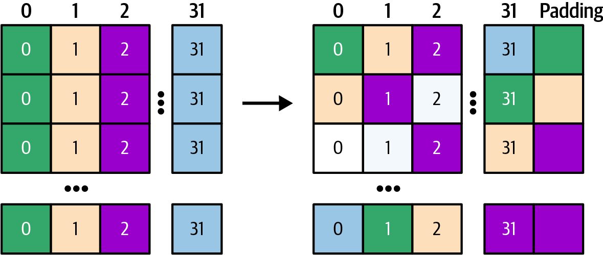
The solution is to adjust data layouts in shared memory to avoid conflicts. A com‐ mon technique is padding shared arrays so that each row, or each memory-access pat‐ tern, maps to different banks. For instance, if you have a 32 × 32 shared tile, you can declare it as [32][33] by adding one extra padding column so that each row now occupies 33 floats. This extra 1-element offset means that when thread k of a warp accesses tile[i][k], successive rows start at addresses that shift across sharedmemory banks. This keeps all threads from hitting the same bank, as shown in Figure 7-6.
Figure 7-6. Avoiding bank conflicts with padding
By changing the stride to 33, no two threads in a warp will contend for the same bank when accessing a given column. This eliminates what would have been a 32-way bank conflict. The padding adds a negligible overhead, ~3% more memory for a 32-wide tile, but it completely eliminates the conflicts, which greatly improves performance. And remember that Blackwell has > 200 KB shared memory per SM. A 3% memory over‐ head is only 1 KB for a 32 × 32 tile. This is worth the performance increase. Let’s show an example of removing shared-memory bank conflicts for a simple trans‐ pose kernel. In this example, each thread accesses shared memory addresses that fall into the same shared-memory bank as other threads. This causes the memory access to serialize, prevents parallelism, and shows slow performance. Here is the native implementation of the transpose kernel that incurs bank conflicts.
Avoid Shared-Memory Bank Conflicts | 267
Before example (C++): naive transpose with bank conflicts:
      #include <cuda_runtime.h>
      #define TILE_DIM 32
      __global__ void transposeNaive(const float *idata, float *odata, int width) {
          __shared__ float tile[TILE_DIM][TILE_DIM];
          int x = blockIdx.x * TILE_DIM + threadIdx.x;
          int y = blockIdx.y * TILE_DIM + threadIdx.y;
           // threads in a warp write a row
           tile[threadIdx.y][threadIdx.x] = idata[y * width + x];
           __syncthreads();
           // Read from shared memory with transposed indices
           // This is a classic case of all threads in a warp
           // hitting the same bank causing a bank conflict
           // Read transposed from shared memory and write out
           odata[x * width + y] = tile[threadIdx.x][threadIdx.y];
      }
      int main() {
          const int N = 1024;
          size_t size = N * N * sizeof(float);
          float *h_idata = (float*)malloc(size);
          float *h_odata = (float*)malloc(size);
          // Initialize input h_idata...
          float *d_idata, *d_odata;
          cudaMalloc(&d_idata, size);
          cudaMalloc(&d_odata, size);
          cudaMemcpy(d_idata, h_idata, size, cudaMemcpyHostToDevice);
           dim3 block(TILE_DIM, TILE_DIM);
           dim3 grid(N / TILE_DIM, N / TILE_DIM);
           transposeNaive<<<grid, block>>>(d_idata, d_odata, N);
           cudaDeviceSynchronize();
           cudaFree(d_idata);
           cudaFree(d_odata);
           free(h_idata);
           free(h_odata);
           return 0;
      }
In this kernel, the tile write into shared memory is row-major (tile[ty][tx]) and therefore coalesced such that each warp writes a full row of 32 floats to shared mem‐ ory in a contiguous manner. (Note: Writing the tile to shared memory with columnmajor tile[tx][ty] would make the warp stride by 128 bytes and trigger a 32-way bank conflict.) In contrast, the tile read is transposed since each thread reads a value where threadIdx.y is the row index and threadIdx.x is the column index.
268 | Chapter 7: Profiling and Tuning GPU Memory Access Patterns
As such, for a given warp, fixed threadIdx.y across threads 0–31, all threads access tile[constant_row][varying_col], meaning the same row index is used across dif‐ ferent columns. This means all 32 addresses are in the same row of the tile array, which occupies a single memory bank segment and causes a 32-way bank conflict. As a result, those reads are serialized by a factor of 32.
                Remember that Blackwell’s shared memory has 32 banks. This num‐
                ber exactly matches the number of threads in a warp, 32. So if all
                threads index into the same bank, as happens when you fix the row
                and vary the column, you will always get a full 32-way conflict. This
                one-to-one correspondence means any misaligned access pattern at
                warp granularity will force every thread to serialize through the same
                bank—regardless of the GPU’s architectural advancements.
In this case, 32 threads attempt to read from 32 different addresses, all in bank 0. This results in heavy serialization of memory accesses and poor performance. Let’s apply padding to remove the conflicts. After example (C++): padded transpose (avoiding bank conflicts). Here, we add a small padding, an extra unused column, so that each row of shared memory starts at a dif‐ ferent bank modulo. This way, the bank-index collisions are eliminated by the offset: #include <cuda_runtime.h> #define TILE_DIM 32 #define PAD 1 // padding columns to avoid bank conflicts
    __global__ void transposePadded(const float *idata, float *odata, int width) {
        // Each row is TILE_DIM+1 elements to shift bank mapping
        __shared__ float tile[TILE_DIM][TILE_DIM + PAD];
        int x = blockIdx.x * TILE_DIM + threadIdx.x;
        int y = blockIdx.y * TILE_DIM + threadIdx.y;
        tile[threadIdx.y][threadIdx.x] = idata[y * width + x];
        // We will optimize this later to use a thread-block-scoped
        // cooperative-groups barrier
        __syncthreads();
        odata[x * width + y] = tile[threadIdx.x][threadIdx.y];
    }
(The host code and setup are the same as in the naive version and omitted for
brevity.)
Avoid Shared-Memory Bank Conflicts | 269
                    PyTorch itself doesn’t expose any high-level APIs for shared-
                    memory padding, so you would have to implement those manually
                    in CUDA kernels and load them with torch.utils.cpp_exten
                    sion). However, in practice, PyTorch relies on optimized libraries
                    like cuDNN and cuBLAS, which implement techniques under the
                    hood to avoid bank conflicts and maximize throughput.
Padding each shared-memory row with an extra element makes each row 33 floats long. Padding by 1 changes the indexing math so that tile[row][col] addresses dif‐ fer in the lower 5 bits for each thread, rather than all threads sharing the same 5-bit bank index. This ensures each thread index maps to a different bank. In the padded kernel, when a warp reads tile[threadIdx.y][threadIdx.x], the addresses for threads 0–31 span multiple banks rather than all hitting bank 0. Now that each thread in the warp accesses distinct banks on reads, bank conflicts are elim‐ inated entirely, as shown in Table 7-5.
Table 7-5. Effect of eliminating shared-memory bank conflicts Metric Before (no padding) After (padding) Shared-memory load bank conflicts 4.8 million 0 Shared-memory utilization (percentage of peak) 52% 100% Warp stall fraction (memory) 38% 0.5% Kernel execution time (ms) 4 ms 1.3 ms (3× improvement)
The Nsight Compute metrics in Table 7-5 confirm the impact: shared-memory load bank conflicts dropped to 0. Shared memory throughput, according to Nsight Com‐ pute, rose from 52% to 100% after eliminating conflicts. The warp stall fraction, the percentage of cycles warps spend stalled on shared-memory reads, dropped from ~38% to near 0%. Here, we have successfully eliminated bank conflicts and unlocked the full perfor‐ mance of the on-chip shared memory. This change improved the kernel’s execution time by about 3× from 4 ms to 1.3 ms since shared-memory accesses went from seri‐ alized to fully parallel. This restores full parallelism for the shared-memory accesses. The cost of padding, 1 extra float per 32, is trivial (~3% memory overhead) compared to the performance gain. An effective alternative to padding is swizzling. Swizzling is a compile-time index transformation that “scrambles” the linear index used for shared memory so that sequential threads map to different banks. For example, one can XOR the index with a bit mask or use a modulo offset to achieve a conflict-free pattern.
270 | Chapter 7: Profiling and Tuning GPU Memory Access Patterns
Swizzling avoids the slight memory overhead of padding while still ensuring perfect bank parallelism. Padding is simpler to implement, but swizzling can achieve the same goal with zero memory overhead—and it’s fun to say!
               NVIDIA’s CUTLASS library and other high-performance CUDA-
               based libraries use index swizzling in their tile iterators to ensure
               threads map to separate banks, avoid bank conflicts, and optimize
               shared-memory usage.
In summary, when using shared memory, it’s important that threads in a warp access different memory banks in parallel rather than queueing up on the same bank. Tech‐ niques like padding and swizzling improve shared-memory load/store efficiency, yielding higher throughput and better performance whenever shared memory is used. Next, let’s explore a technique to avoid shared memory altogether and communicate directly between threads.
Warp Shuffle Intrinsics: Avoid Shared Memory and Explicit Synchronization The preceding avoiding-bank-conflicts technique assumes that we use shared mem‐ ory for communication between threads. But what if we could avoid shared memory altogether—and its bank conflict issues? NVIDIA GPUs support warp-synchronous primitives that allow threads in the same warp to exchange data through registers instead of shared memory. In fact, these primitives work only within a single warp such that threads exchange data with their 31 siblings. So no memory banks are involved for this intrawarp communication— and therefore no bank conflicts are possible. The most common are the __shfl_sync intrinsics (shuffle). __shfl_sync lets you broadcast a value from one thread to all other threads in a warp. You can also per‐ form warp-level reductions without ever writing to shared memory. And remember that these intrinsics let threads exchange values through registers (instead of shared memory), which completely eliminates shared-memory bank conflicts.
               Modern GPUs will automatically broadcast a single shared-
               memory value if all threads access the exact same memory address.
               This will avoid a bank conflict in this special, single-address case.
               Warp shuffles, on the other hand, use broadcasting to avoid bank
               issues for the more general, arbitrary, multivalue pattern of data
               access.
Warp Shuffle Intrinsics: Avoid Shared Memory and Explicit Synchronization | 271
Imagine you need to sum the 32 per-thread partial results within a single warp. The naive shared-memory approach would have each thread write its value into a shared array, call a synchronization barrier, and then read and accumulate all 32 entries. This risks bank conflicts and adds additional synchronization overhead. With __shfl_sync, you can do a tree-style reduction entirely in registers. For exam‐ ple, let’s use a convenience variant called __shfl_down_sync to perform a butterflystyle reduction such that each thread reads the value held by another thread that is offset a number of lanes away, as shown here: unsigned mask = __activemask(); float val = threadVal; // each thread’s partial sum
      // Perform butterfly reduction: exchange values with increasingly distant lanes
      for (int offset = 16; offset > 0; offset >>= 1) {
          float other = __shfl_down_sync(mask, val, offset);
          val += other;
      }
// After the loop, lane 0 holds the warp’s total sum
Here, each __shfl_down_sync directly reads another lane’s register, halving the active threads each step, until lane 0 accumulates the full sum. Because all communication stays in registers, there’s no shared-memory traffic and thus zero bank conflicts or extra synchronizations. In short, __shfl_sync and its variants perform operations entirely within the warp’s execution lanes. This avoids bank conflicts because no shared memory is used. And it’s often faster since it uses registers and cuts down on the number of sharedmemory instructions. Many high-performance warp-level reductions bypass shared memory entirely by using shuffle intrinsics, which exchange values directly through registers in just a few instructions and incur no bank conflicts. CUDA’s Cooperative Groups API builds on these primitives. This API provides calls like thread_group.shuffle() to simplify intrawarp communication. Helper intrinsics like __reduce_sync() ultimately com‐ pile down to these shuffle patterns for intra-warp data exchange on modern NVIDIA GPUs.
                    Shuffles work within a single warp only. For interwarp exchange on
                    modern GPU architectures, also consider thread-block-wide
                    reductions using cooperative groups or thread-block-cluster-level
                    communication when supported. We will discuss these concepts in
                    Chapter 10.
272 | Chapter 7: Profiling and Tuning GPU Memory Access Patterns
Remember, however, that shuffles are limited to the 32 threads within a single warp. Whenever you need to pass data across warps, you must still fall back on shared or global memory with proper synchronization. In Chapter 10, we’ll explore interwarp patterns like cooperative group (CG) synchro‐ nization primitives, multiwarp shuffle methods, and thread block clusters (CTA clus‐ ters). All of these ultimately use the same hardware intrinsics under the hood. Mastering both intrawarp and interwarp techniques is essential because memoryrelated bottlenecks remain one of the most common causes of GPU performance issues.
Read-Only Data Caches When all threads read the same values or a thread rereads data that does not change, failing to use the GPU’s caching mechanisms can bottleneck performance. For exam‐ ple, consider a large lookup table such as an embedding vector in a natural language processing (NLP) model that is read-only during inference. Many threads might need to access this vector in parallel. A naive implementation might fetch from global memory each time, even though the data is immutable and could be cached on-chip. Note that the read-only cache we refer to here is different from the 64 KB constant memory cache discussed previously in the GPU memory hierarchy section. It’s a large cache for immutable data. The constant memory cache, on the other hand, is too small for big arrays. Modern architectures rely on the larger L1/read-only cache for these types of embedding-vector lookups—rather than trying to squeeze this data into the small 64 KB constant memory cache. On modern GPUs, global memory loads are automatically cached in L2 and often L1. You can use const __restrict__ qualified pointers to define your function argu‐ ments as non-coherent and read-mostly (versus read-only). For read-only data, the compiler may route loads through this read-only path when it can prove immutabil‐ ity, nonaliasing, and safety. This lets the compiler/hardware route unchanging data through the read-only L1 cache, which has lower latency—especially for broadcast accesses—and doesn’t evict other cached data.
               In modern CUDA, you usually don’t need to call __ldg() explicitly.
               If a pointer is const __restrict__, the compiler may use the read-
               only data cache for global memory loads when it can provide
               safety. The older __ldg() intrinsic is still available for explicit con‐
               trol, but it’s generally not needed with modern compilers.
A common performance pitfall is forgetting to tell the compiler that a buffer is truly read-only, which means it won’t use the read-only (non-coherent) data path and won’t route those loads through the specialized read-only cache. Instead, every access
Read-Only Data Caches | 273
becomes a plain global memory load, resulting in redundant DRAM traffic and spu‐ rious cache misses. When you profile such a kernel, you’ll spot the same addresses fetched repeatedly from off-chip memory, see no __ldg() operations in the instruction stream, observe a surprisingly low L2 hit rate for that array, and measure elevated DRAM throughput reminiscent of an uncached workload. The solution is to leverage the read-only path by marking data as const __restrict__ , or by explicitly using the __ldg() intrinsic to load it. This tells the hardware that the data will not be modified, allowing it to be cached in the specialized read-only cache, which sits alongside L1 and has lower latency for broadcast loads. When a warp issues a constant‐cache load (__constant__ or uniform __ldg() in older GPUs), the hardware can service all 32 lanes with a single transaction if they hit the same address. By broadcasting that value to every thread, it uses only one cycle instead of doing 32 separate loads. This warp-wide broadcast reduces both latency and memory bandwidth usage for uniform data like lookup tables, coefficients, etc. This lets you fetch a shared constant, for free essentially, once per warp rather than 32 times per warp (1 per thread). As an example of caching benefits using the standard read-only cache, suppose we have a kernel that, for each thread, looks up a value from a table of size T = 1,024 and writes it to an output. This simulates an embedding-lookup pattern and is shown here in both CUDA C++ and PyTorch: #include <cuda_runtime.h> #define T 1024
      __global__ void naiveLookup(const float* table, float* out, int N) {
          int idx = blockIdx.x * blockDim.x + threadIdx.x;
          if (idx < N) {
              // __ldg not used here, each access goes to
              // global memory without using read-only cache
              int t = idx % T;
              out[idx] = table[t];
          }
      }
      int main() {
          const int N = 1 << 20;
           float* h_table = nullptr;
           float* h_out = nullptr;
           cudaMallocHost(&h_table, T * sizeof(float));
           cudaMallocHost(&h_out, N * sizeof(float));
for (int i = 0; i < T; ++i) h_table[i] = float(i);
274 | Chapter 7: Profiling and Tuning GPU Memory Access Patterns
        float *d_table, *d_out;
        cudaMalloc(&d_table, T * sizeof(float));
        cudaMalloc(&d_out, N * sizeof(float));
        cudaMemcpy(d_table, h_table, T * sizeof(float),
            cudaMemcpyHostToDevice);
        dim3 block(256), grid((N + 255) / 256);
        naiveLookup<<<grid, block>>>(d_table, d_out, N);
        cudaDeviceSynchronize();
        cudaMemcpy(h_out, d_out, N * sizeof(float), cudaMemcpyDeviceToHost);
        cudaFree(d_table);
        cudaFree(d_out);
        cudaFreeHost(h_table);
        cudaFreeHost(h_out);
        return 0;
    }
Here is a rough PyTorch equivalent to the naive version shown in CUDA C++:
    import torch
    def vectorized_lookup(table, N):
        flat = table.view(-1)
        T = flat.size(0)
        # build indices [0,1,2,...,N-1] % T all on GPU
        idx = torch.arange(N, device=flat.device) % T
        # one gather kernel does all N loads in parallel
        return flat.index_select(0, idx)
    # Usage
    T = 1024
    N = 1 << 20
    table = torch.arange(T, dtype=torch.float32,
                         device='cuda')
    out = vectorized_lookup(table, N)
In these naive versions, each lookup likely hits in L2 after the first use (since L2 will
cache it), but there is no use of the specialized read-only cache. The hardware may
still treat it as normal global data, which could evict other useful data or not take full
advantage of broadcast caching if multiple threads read the same table[t] in a warp.
Now we optimize the kernel by marking the table as const __restrict__. This will
hint to the hardware that it should use the read-only cache path, which is shown here:
    #include <cuda_runtime.h>
    #define T 1024
    __global__ void lookup(const float* __restrict__ table,
            float* out, int N) {
Read-Only Data Caches | 275
           int idx = blockIdx.x * blockDim.x + threadIdx.x;
           if (idx < N) {
               int t = idx % T;
               // Compiler can turn this into a load from the
               // read-only cache for faster loads
               out[idx] = table[t];
           }
      }
      int main() {
          const int N = 1 << 20;
           float* h_table = nullptr;
           float* h_out = nullptr;
           cudaMallocHost(&h_table, T * sizeof(float));
           cudaMallocHost(&h_out, N * sizeof(float));
for (int i = 0; i < T; ++i) h_table[i] = float(i);
           float *d_table, *d_out;
           cudaMalloc(&d_table, T * sizeof(float));
           cudaMalloc(&d_out, N * sizeof(float));
           cudaMemcpy(d_table, h_table, T * sizeof(float), cudaMemcpyHostToDevice);
           dim3 block(256), grid((N + 255) / 256);
           lookup<<<grid, block>>>(d_table, d_out, N);
           cudaDeviceSynchronize();
           cudaMemcpy(h_out, d_out, N * sizeof(float), cudaMemcpyDeviceToHost);
           cudaFree(d_table);
           cudaFree(d_out);
           cudaFreeHost(h_table);
           cudaFreeHost(h_out);
           return 0;
      }
                    In a PyTorch setting, you could implement the same trick by writing
                    a small CUDA extension with torch.utils.cpp_extension that
                    declares your embedding table pointer as const __restrict__. You
                    could also use the PyTorch compiler to optimize this code. We’ll
                    cover the PyTorch compiler in depth in Chapters 13 and 14.
In short, marking the table const __restrict__ tells the compiler that these values are immutable and not aliased, which permits the use of the read-only data path when safe to do so. This increases cache hit rate and reduces off-chip traffic. Table 7-6 shows Nsight Compute measurements before and after this change.
276 | Chapter 7: Profiling and Tuning GPU Memory Access Patterns
Table 7-6. Benefit of read-only cache Metric Before (no __restrict__) After (__restrict__ used) Global Memory Load Efficiency 52% 97% DRAM throughput (GB/s) 600 GB/s 200 GB/s L2 read throughput (GB/s) 1,500 GB/s 1,800 GB/s SM Active % 45% 93% Kernel execution time (ms) 2.5 ms 1.0 ms
After adding const __restrict__, the kernel time improves by about 2.5×, from 2.5 milliseconds to 1.0 millisecond, because warps spend less time stalled on DRAM. SM Active % rises from 45% to 93%, indicating that nearly every cycle has active work rather than idle memory waits. DRAM throughput falls from 600 GB/s to 200 GB/s, while L2 read throughput increases from 1,500 GB/s to 1,800 GB/s as more requests are satisfied in cache. Global Memory Load Efficiency increases from 52% to 97%, confirming that most fetched cache lines carry useful data.
                    Nsight Systems presents a timeline view of overall GPU activity,
                    while Nsight Compute reports per-kernel metrics such as SM
                    Active %. Use Nsight Compute when you need quantitative per-
                    kernel analysis.
Because more traffic is served by on-chip caches rather than traveling to DRAM, the compute units remain fed and arithmetic intensity increases. This balance is what moves a kernel from the memory-bound regime toward the compute-bound regime. Texture objects and surface objects are also available for read-only and read/write access patterns with strong two-dimensional or three-dimensional locality. By bind‐ ing an array to a cudaTextureObject_t and using tex1Dfetch or tex2D fetches, the hardware can exploit spatial locality with high cache hit rates and features such as wrapping and interpolation. Surface objects allow writes on similar access patterns.
                    While texture reference and surface reference APIs are deprecated,
                    texture object and surface object APIs remain supported and are
                    appropriate for access patterns with two- or three-dimensional
                    locality. However, for most AI workloads involving 1D data, using
                    the read-only data cache with constant memory is much simpler
                    and preferred.
In summary, mark read-only data as const __restrict__ to tap into the low-latency read-only cache, cutting DRAM traffic and lifting SM activity. Consider texture or surface memory whenever your access pattern has 2D/3D locality that a regular cache
Read-Only Data Caches | 277
might not handle optimally. Together, these techniques collapse memory stalls, boost cache utilization, and unlock substantial performance gains for memory-bound kernels.
Asynchronous Memory Prefetching and Tensor Memory Accelerator In earlier sections, we saw how coalescing dozens of 4-byte loads into a single 128byte transaction significantly improved global-load efficiency and cut wasted sectors per request. Yet even a perfectly coalesced load still stalls a warp for the full DRAM round trip. On Blackwell, for instance, a full DRAM round-trip is on the order of hundreds of cycles before any computation can begin. To hide that latency, we need to overlap data transfer with compute. This overlap is what hides most of the DRAM latency. CUDA’s Pipeline API together with the Tensor Memory Accelerator (TMA) hardware engine take this idea to the thread-block level. Instead of having each warp use the SM’s load and store (LD/ST) units to fetch data from global memory, you can invoke the TMA engine to asynchronously fetch an entire tile from global memory into shared memory, as shown in Figure 7-7.
Figure 7-7. TMA asynchronously fetching data from global HBM into shared memory
To start the TMA transfer, you can call cuda::memcpy_async(). On modern GPU architectures, cuda::memcpy_async() together with cuda::pipeline exposes the hardware engines for asynchronous global to shared transfers. This includes the TMA when available. This will use TMA’s on-chip DMA engine to perform the asyn‐ chronous bulk data transfer. This is implemented in CUDA as follows:
278 | Chapter 7: Profiling and Tuning GPU Memory Access Patterns
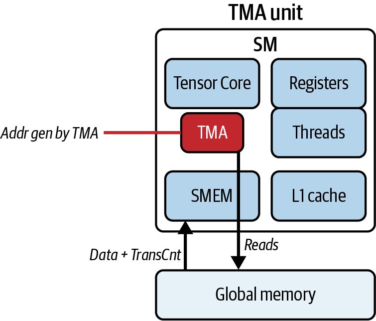
cuda::memcpy_async(sharedBuf, globalPtr + offset, cuda::aligned_size_t<16>(bytes), pipe); pipe.producer_commit(); And while TMA handles the bulk copy, including coalescing, strided transfers, and even multidimensional transfers, the kernel computes the previous tile. This is called double buffering, or ping-ponging. By implementing double buffering with TMA, the SM’s load/store units are now free to do real work because TMA’s DMA engine moves data for us in the background. In effect, data movement becomes asynchronous such that while TMA streams in the next tile of data, the SM’s warps compute on the previous tile. This overlap is what hides the 800-cycle DRAM latency. Specifically, TMA is capable of 1D–5D bulk copies and arbitrary strides between global and shared memory without blocking the SM instruction pipeline. By offload‐ ing these transfers from the SM to TMA, your kernel issues far fewer LD/ST instruc‐ tions, eliminates extra synchronization, and lets the warp schedulers spend almost every cycle on useful computation instead of waiting on memory. Here is a code snippet showing how to initiate an asynchronous copy from global to shared memory using the CUDA C++ Pipeline API and the TMA hardware engine: #include <cuda/pipeline> #include <cuda_runtime.h> #include <cstdint> #include <cassert>
    #define TILE_SIZE 1024 // example tile size
    // User-provided compute function operating on a shared-memory tile
    __device__ void processTile(const float* tile);
    __global__ void kernelWithTMA(const float* __restrict__ global_ptr,
                                  int nTiles) {
        // Two ping-pong buffers in shared memory
        // On Blackwell (CUDA 13+), prefer 32B alignment for 256-bit vectors
        // (v8.f32 / double4).
        __shared__ __align__(VEC_BYTES) float tile0[TILE_SIZE];
        __shared__ __align__(VEC_BYTES) float tile1[TILE_SIZE];
float* tiles[2] = { tile0, tile1 };
        // Alignment / size guards for vectorized copies
        // --- choose vector width -------------------------------------------------
        #ifndef VEC_BYTES
          // Prefer 32B vectors on CUDA 13+/Blackwell.
          // Define -DUSE_256B_VEC to force.
          #if defined(USE_256B_VEC) || (defined(CUDA_VERSION)&&CUDA_VERSION >= 13000)
            #define VEC_BYTES 32      // 256-bit: v8.f32, double4
Asynchronous Memory Prefetching and Tensor Memory Accelerator | 279
             #else
               #define VEC_BYTES 16       // 128-bit: v4.f32, float4
             #endif
           #endif
           constexpr int VEC_ELEMS = VEC_BYTES / sizeof(float); // 4 (128b) or 8 (256b)
           constexpr int WARP       = 32;
           // Alignment / size guards for vectorized copies/compute
           static_assert((TILE_SIZE % (WARP * VEC_ELEMS)) == 0,
                         "TILE_SIZE must be a multiple of WARP_SIZE * VEC_ELEMS");
           // Also guarantee the tile byte count
           // is a multiple of the vector width
           static_assert(((TILE_SIZE * sizeof(float)) % VEC_BYTES) == 0,
                         "Tile byte size must be a multiple of VEC_BYTES");
           // On Blackwell (CUDA 13+), prefer 32B alignment
           // for 256-bit vectors (v8.f32 / double4).
assert((reinterpret_cast<std::uintptr_t>(global_ptr) % VEC_BYTES) == 0);
           size_t bytes = TILE_SIZE * sizeof(float);
           // Block-scoped pipeline for TMA
           __shared__ cuda::pipeline_shared_state<
               cuda::thread_scope_block, 2> state;
           auto pipe =
               cuda::make_pipeline(cuda::this_thread_block(),
                   &state);
           // Prime pipeline with the first async copy into tile0
           pipe.producer_acquire();
           cuda::memcpy_async(tiles[0],
                              global_ptr + 0 * TILE_SIZE,
                              cuda::aligned_size_t<32>{bytes},
                              pipe);
           pipe.producer_commit();
           // Loop over the remaining tiles
           for (int t = 1; t < nTiles; ++t) {
               // Wait for the previous copy to finish, then compute on it
               pipe.consumer_wait();
               processTile(tiles[(t - 1) & 1]);
               pipe.consumer_release();
                // Enqueue the next async copy into the alternate buffer
                pipe.producer_acquire();
                cuda::memcpy_async(tiles[t & 1],
                                   global_ptr + t * TILE_SIZE,
                                   cuda::aligned_size_t<32>{bytes},,
                                   pipe);
                pipe.producer_commit();
           }
280 | Chapter 7: Profiling and Tuning GPU Memory Access Patterns
       // Final wait and compute on the last tile
       pipe.consumer_wait();
       processTile(tiles[(nTiles - 1) & 1]);
       pipe.consumer_release();
   }
Immediately after kernel launch, each block allocates two shared-memory tiles
(tile0, tile1) and constructs a block-scoped pipeline so all threads in the thread
block coordinate their asynchronous DMA, as shown here:
   __shared__ cuda::pipeline_shared_state<
       cuda::thread_scope_block, 2> state;
auto pipe = cuda::make_pipeline(cuda::this_thread_block(), &state); To prime the pipeline, we submit an asynchronous copy using the TMA, which coa‐ lesces even strided or multidimensional transfers and streams bytes from global memory into tiles[0] in the background, as seen here: pipe.producer_acquire(); cuda::memcpy_async(tiles[0], global_ptr + 0 * TILE_SIZE, cuda::aligned_size_t<32>{bytes}, pipe); pipe.producer_commit(); Before using that data, we do the following to ensure we block just long enough for the TMA to finish the copy: pipe.consumer_wait(); processTile(tiles[0]); pipe.consumer_release();
Inside the main loop, we alternate buffers using pipe.consumer_wait(); + process Tile() on the previous tile, pipe.consumer_release(), pipe.producer_acquire() + new cuda::memcpy_async() into the other tile, and pipe.producer_commit(). Then we repeat! By ping-ponging between tile0 and tile1, each new memcpy_async overlaps processTile on the previous buffer. The load and store units on the SM experience lower pressure with more instruction issue slots available for computation. At the same time, the TMA moves data in parallel. This eliminates redundant global mem‐ ory loads, reduces synchronization overhead, and keeps warps busy rather than stal‐ led on memory. Asynchronous prefetching from global memory to shared memory hides latency behind compute. Threads preload upcoming data into shared memory while they compute on data that was previously loaded.
Asynchronous Memory Prefetching and Tensor Memory Accelerator | 281
This pattern is especially effective in memory-bound loops and tensor computations. On modern GPUs, the TMA can stream the next tile for a matrix multiply while the current tile is being processed.
                    TMA is the preferred path for tiled bulk copies when moving 2D
                    and N-dimensional tiles between global memory and SMEM/
                    TMEM. Prefer cuda::memcpy_async with cuda::pipeline at block
                    scope; on Hopper/Blackwell the implementation will leverage TMA
                    (cp.async.bulk.* family) when alignment and direction permit
                    (e.g., global memory ↔ shared memory).
We trade many scattered global reads for one coalesced global copy plus many fast shared-memory loads. This is favorable given the gap between DRAM and on-chip SRAM. Table 7-7 summarizes Nsight Compute metrics before and after a TMA-based double-buffering implementation.
Table 7-7. Comparing naive kernel (no prefetch) to TMA-accelerated double buffering Metric Before (no prefetch) After (async prefetch) Global Memory Load Efficiency 23% 99% Average sectors per request 6.4 4.0 DRAM throughput (% of peak) 25% 90% SM Active % 62% 100% Kernel execution time 18 ms 7 ms
Here, we see SM Active % approaches 100%, which shows that the SMs have active warps for nearly all cycles. Global Memory Load Efficiency increases from 23% to 99%, meaning nearly every fetched byte is useful. Average sectors per request falls from 6.4 to about 4.0, which indicates that requests map cleanly to 128-byte lines at the cache. DRAM throughput rises from 25% to 90% of peak, and overall time improves from 18 milliseconds to 7 milliseconds, about 2.6× faster. These results confirm that offloading bulk copies to the TMA and pingponging shared memory buffers keep the GPU busy and hide most of the DRAM latency behind useful work. NVIDIA’s CUDA pipeline API plus TMA is a textbook example of hardwaresoftware codesign. The Pipeline API specifically exposes TMA’s capabilities—and the TMA hardware supports exactly the asynchronous, coalesced, multidimensional copies that cuda::memcpy_async needs. The API and the TMA DMA engine were developed hand in hand so you can express high-level pipeline operations that map closely to the hardware transfer capabilities.
282 | Chapter 7: Profiling and Tuning GPU Memory Access Patterns
This allows the efficient overlap of memory movement with compute to boost performance.
               For almost all cases, you should write your CUDA kernels with the
               highest-level and most-recent APIs available for global-to-shared
               tiling. This includes the CUDA Pipeline API (cuda::mem
               cpy_async). These APIs and libraries are constantly improving and
               will transparently leverage the latest hardware features like TMA
               for bulk, strided, and 2D/3D transfers. In addition, they enable
               advanced performance optimization features like multicast with
               thread block clusters. When using these APIs, you get all of this
               “for free"-without requiring code changes.
In summary, when memory access limits your kernel’s performance, offload and overlap data movement by combining careful tiling, double buffering, and TMAdriven asynchronous prefetching. By staging tiles in shared memory and using cuda::memcpy_async alongside pipe.producer_commit and pipe.consumer_wait, you hand off coalesced, multidimensional DMA transfers to the TMA, offloading the global to shared memory transfer. Using TMA to offload memory transfers helps to relieve pressure on the SM’s load/ store units to help keep the computation pipeline full. As such, the SM focuses on compute, while shared memory traffic uses the on-chip TMA path. On Blackwell’s massive-bandwidth HBM3e fabric, these techniques are essential to hide DRAM latency, sustain peak throughput, and turn memory-bound kernels into nearcompute-bound workhorses.
Key Takeaways
Optimizing memory access patterns on GPUs—through coalescing, data reuse, and
asynchronous transfers—can shift a kernel from being memory bound to approach‐
ing the hardware’s peak capabilities. Small code changes to better align with GPU
architecture (such as proper thread grouping, using shared memory, avoiding bank
conflicts) can yield massive performance gains. Here are the key takeaways from this
chapter:
Global-memory coalescing
    Coalescing is achieved when each warp’s accesses fall within as few 128-byte cache
    lines as possible. Arrange your data and thread indexes so that each warp’s threads
    read consecutive 4-byte words, letting the hardware fuse them into a few 128-byte
    transactions. Coalesced memory loads maximize effective DRAM bandwidth, or
    Global Memory Load Efficiency, and minimize average sectors per request down
    to the optimal 4.0 value. When using modern versions of Nsight Compute, you can
Key Takeaways | 283
      also use sm__sass_data_bytes_mem_* counters and gpu__dram_throughput
      .avg.pct_of_peak_sustained_elapsed to profile and optimize memory
      coalescing.
Vectorized loads/stores
    Use built-in vector types such as float4 for 16-byte vectors. On Blackwell with
    CUDA 13+, prefer 32-byte per-thread vectors when 32-byte alignment is prova‐
    ble. This includes double4 or a custom struct alignas(32) { float v[8]; }.
    This reduces instructions per byte and keeps sectors/request at the ideal 4.0 when
    properly aligned. This way, each thread moves as many elements as possible in
    one instruction. The number of 128-byte transactions per warp scales with the
    total bytes requested. Be mindful of alignment: ensure your arrays are allocated
    with at least 16-byte alignment for float4, which cudaMalloc does by default
    using 256-byte alignment, typically. Misaligned vector accesses will forfeit these
    benefits.
Bank-conflict avoidance
   Pad your shared-memory arrays (e.g., make rows 33 floats wide for 32-thread
   warps) so that no two threads hit the same bank in the same cycle. Removing
   bank conflicts restores full shared-memory throughput. Try swizzling for a
   slightly more memory-efficient implementation than padding.
Shared-memory tiling and data reuse
    Stage working sets in on-chip shared memory (e.g., tiling a matrix in 32 × 32
    blocks) so each element is fetched once from DRAM but used many times on the
    SM. This raises arithmetic intensity and shifts kernels toward being compute
    bound.
Read-only data cache
   Mark small, static lookup tables or coefficients as const __restrict__ so the
   compiler can route loads through the read-only data path when applicable. Uni‐
   form broadcasts are lower-latency than DRAM, avoid redundant transactions,
   and can be served from on-chip cache.
Overlap host–GPU copies with streams
   Allocate your host buffers as page-locked (“pinned”) memory, and use cuda
   MemcpyAsync on multiple streams to overlap H2D/D2H transfers with kernel exe‐
   cution. Pinned memory enables asynchronous DMA transfers, and multiple
   streams allow copies to overlap with kernel execution to hide PCIe or NVLink
   transfer latency. Prefer cudaMemcpyAsync with explicit streams and events to
   overlap H2D/D2H and kernels. Remember that pageable (non-pinned) memory
   will disable DMA overlap. You should verify whether pageable or pinned mem‐
   ory is used, as observed transfer rates will vary widely depending on this
   configuration.
284 | Chapter 7: Profiling and Tuning GPU Memory Access Patterns
Asynchronous prefetch with TMA + Pipeline API
    Use the C++ libcu++ barrier and pipeline APIs (cuda::barrier and cuda::pipe
    line) with cuda::memcpy_async to drive TMA (cp.async.bulk.tensor) for
    global memory → shared memory bulk copies when alignment and scope
    requirements are met. This offloads coalesced, strided (even multidimensional)
    copies into shared memory and overlaps them with computation with double
    buffering. This will reduce pressure on the SM’s LD/ST units and let the SM
    focus on compute.
    It’s important to note that the libcu++ pipeline APIs and TMA continue to
    evolve. Prefer the staged forms (e.g., producer_acquire(), producer_commit(),
    consumer_wait(), consumer_release()) for two-stage ping-pong buffers. Use a
    block-scoped pipeline (e.g., cuda::thread_scope_block) or block-scoped barrier
    (e.g., cuda::barrier<cuda::thread_scope_block>) unless you specifically need
    cluster-scoped or grid-scoped copies.
Profile to guide you
    Rely on Nsight Compute metrics like Global Memory Load Efficiency, average
    sectors per request, shared-memory bank conflicts, SM Active %, warp stall rea‐
    sons, etc. Also, review Nsight Systems timelines to visualize overlaps and stalls,
    pinpoint bottlenecks, and verify each optimization.
Conclusion With your memory-access pipeline now firing on all cylinders with coalesced global memory loads, conflict-free tiling, vectorized fetches, read-only caching, and TMAdriven prefetching, you’ve removed the biggest data-movement bottlenecks and freed the SMs to run at full speed. Throughout this chapter we’ve relied on Nsight Compute and Nsight Systems to expose exactly where warps were starving for data. We also used them to confirm, step by step, that each optimization really did reduce stalls, collapse wasted transac‐ tions, and boost sustained bandwidth. Those tools remain your north star whenever you tune a new kernel. In the next chapter, we’ll cover some fundamental latency-hiding techniques in CUDA and GPU programming. These techniques include tuning occupancy, increas‐ ing warp efficiency, avoiding warp divergence, and exposing instruction-level parallelism.
Conclusion | 285