Ch 8 — Occupancy Tuning, Warp Efficiency, and Instruction-Level Parallelism
Modern GPU-accelerated workloads are pushing hardware to its limits. Multi-die GPUs like Blackwell connect multiple reticle-limited dies with a 10 TB/s NV-HBI link and increase L2 to 126 MB. These hardware design choices materially change memory-vs-compute tradeoffs and occupancy sweet spots. This makes profiling and optimization even more critical than ever. Building on the fundamentals of memory optimizations, we now turn to advanced latency-hiding techniques and throughput enhancements designed to fully leverage the full power of modern GPUs. We will focus on identifying performance bottlenecks and then applying a systematic set of optimization strategies to eliminate them one by one. Key themes in this chap‐ ter include tuning occupancy, optimizing warp efficiency, and increasing instructionlevel parallelism. By the end of the chapter, you will be able to identify root causes of GPU underutilization—as well as apply the right combination of optimizations. We will also prepare you for more advanced techniques like kernel fusion and pipelining with primitives like CUDA Graphs and CUDA streams, which we cover in subsequent chapters. While our focus is higher-level languages like CUDA C++ and AI frameworks like PyTorch, the principles of profiling and tuning apply at all levels of the stack right down to the hardware. As such, understanding low-level hardware performance remains critical for diagnosing bottlenecks that higher-level abstractions make diffi‐ cult to fully resolve.
Profiling and Diagnosing GPU Bottlenecks Before optimizing, we must first identify the bottlenecks in our code to determine which hardware or software resource is limiting our performance. Modern NVIDIA GPUs are complex, and a slowdown could come from many sources, including mem‐ ory bandwidth, memory latency, instruction throughput, synchronization overheads, insufficient parallelism, host-device transfer delays, and more. NVIDIA’s profiling ecosystem includes Nsight Systems (command-line interface nsys) and Nsight Compute (command-line interface ncu). Nsight Systems captures a system-level timeline of CPU threads, GPU kernels, and memory transfers. It can also capture Python backtraces and Python sampling. Combined with PyTorch profiler and various visualization tools, Nsight Systems and Nsight Compute can help you diagnose kernel performance bottlenecks, analyze roofline plots, and measure the effectiveness of your iterative optimization efforts.
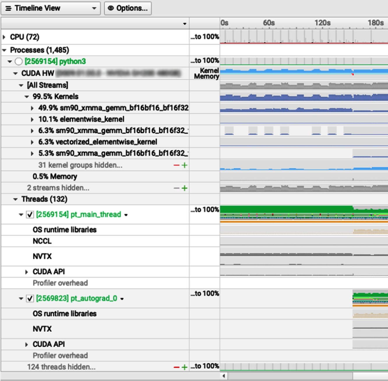
Nsight Systems Timeline View The Nsight Systems timeline view helps pinpoint concurrency issues, transfer over‐ head, and idle periods. For example, run the following code to produce a detailed timeline showing kernel launch overlaps, CPU preparation gaps, data transfer tim‐ ings, and NVTX-marked ranges: nsys profile \ --trace=... \ --capture-range=... \ --force-overwrite=true \ <application> In addition, the Nsight Systems GUI lets you interactively inspect the timeline. It vis‐ ualizes CPU threads, GPU kernels, and even user-defined NVTX ranges with zoom and pan features for detailed analysis (see Figure 8-1). Remember that NVTX annotations are essential for complex applications. Use NVTX ranges in your code to mark regions of interest. You can then use Nsight Systems to capture range profiles. And while the CUDA profiler Start and Stop API is supported for capture control, NVTX ranges are the recommended mechanism for framework workflows. For instance, you can use NVTX range push/pop, available using torch.cuda.nvtx in PyTorch, to label phases such as “forward pass” and “backprop.” This makes the Nsight Systems timeline far more interpretable since the profiler can capture the performance-critical iterations and clearly delineate key computation segments.
288 | Chapter 8: Occupancy Tuning, Warp Efficiency, and Instruction-Level Parallelism
Figure 8-1. Nsight Systems interactive UI (source: https://oreil.ly/YEiWS)
Profiling and Tuning the Data Pipeline As mentioned earlier, Nsight Systems provides a high-level view of the entire pipeline, including the data loading and processing steps. For instance, if you see the GPU idle while the CPU is busy preparing data or running augmentation, common in training loops, the bottleneck might not be the GPU kernel but the data pipeline itself. For scenarios in which the bottleneck is the data pipeline on a realistic and represen‐ tative dataset, you can tune the number of data loader threads, overlap CPU prepro‐ cessing with GPU compute using double buffering, or move more preprocessing onto the GPU.
Profiling and Diagnosing GPU Bottlenecks | 289
                     Always ensure that what you perceive as a “GPU performance
                     issue” is not actually caused by something upstream or down‐
                     stream of the kernel execution like data loading.
With a clear picture from profiling, we can now proceed to address specific bottle‐ necks. The next sections cover the core optimization techniques in detail. We’ll start with occupancy tuning since a sufficient supply of warps is fundamental to hiding latency and maximizing throughput.
Nsight Compute and Roofline Analysis Nsight Compute (ncu), on the other hand, is a profiler that collects in-depth metrics for individual kernels. For instance, it tracks achieved occupancy, issued warp instructions per cycle, memory throughput (GB/s), utilization of execution units, and many others. Together, these paint a complete picture of your system’s performance profile. These metrics are organized into sections such as memory, compute, and throughput, etc. Nsight Compute’s automated analysis rules will flag inefficiencies such as lowmemory utilization and divergent branches—and even provide optimization hints. These built-in rules are updated continuously for new GPU architectures. They can quickly highlight if you are memory bound, latency bound, etc., based on metrics like FLOPS per byte ratios, stall reasons, etc. Nsight Compute includes a Roofline analysis section as well as automated guidance. This can plot your kernel’s achieved FLOPS against hardware rooflines—and even highlight if you are near the memory bandwidth or compute limits. Remember that the memory-versus-compute distinction is quantified using the Roof‐ line model, which plots kernel performance against hardware ceilings for memory bandwidth and compute throughput. Nsight Compute now directly provides Roof‐ line analysis, showing each kernel’s achieved GFLOPS relative to peak and its arith‐ metic intensity (FLOPS per byte). A kernel falling below the memory roof indicates memory-bound behavior, while one near the compute roof is ALU bound. Use the Roofline section in Nsight Compute to obtain arithmetic intensity (FLOPs/byte) and FLOPs by precision directly. Compare this to the hardware’s theoretical peak FLOPS per byte, you can see how far below the roofline the kernel is operating. An example Roofline chart is shown in Figure 8-2.
290 | Chapter 8: Occupancy Tuning, Warp Efficiency, and Instruction-Level Parallelism
Figure 8-2. Roofline chart shown in the Nsight Compute UI (https://oreil.ly/wUbIz)
It’s often effective to first use Nsight Systems to find hot kernels or bottleneck opera‐ tions on the timeline. Then, you can zoom into each of these kernels with Nsight Compute to perform a more fine-grained analysis and diagnosis. This two-step work‐ flow, moving from a system-wide view to a kernel-level deep dive is a common approach to handling complex GPU performance debugging and tuning.
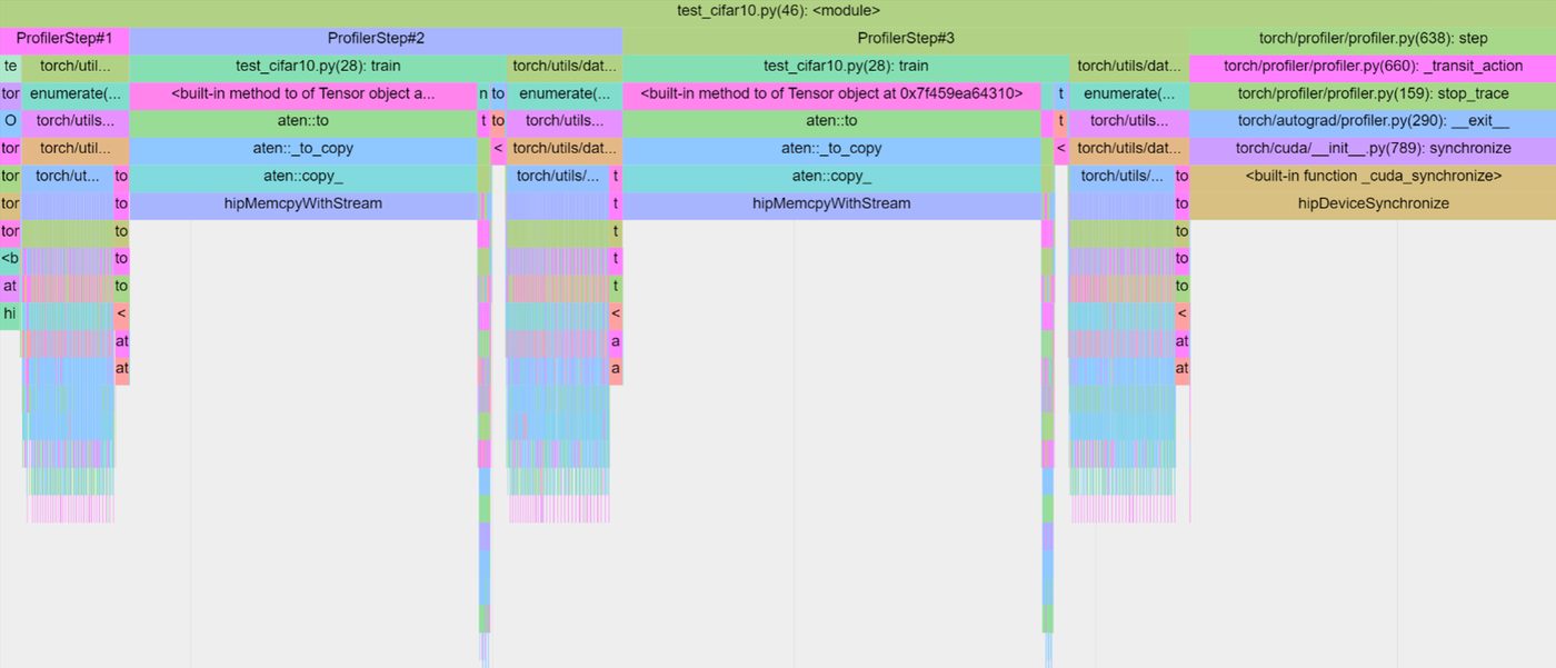
PyTorch Profiler and Visualization Tools When using high-level frameworks like PyTorch, the torch.profiler API can collect similar performance metrics during model training/inference. The PyTorch profiler uses the Kineto library to actually perform the data collection under the hood. Kineto integrates with CUDA’s Performance Tools Interface (CUPTI) backend to cap‐ ture operator-wise execution times, GPU kernel launches, memory copies, and hard‐ ware counter metrics. It also integrates with Linux perf to record CPU events. Kineto merges all of this information into a coherence, time-ordered trace, which can be visualized using the PyTorch profiler UI, Nsight Systems GUI, or just a Chrome browser (e.g., Chrome tracing format). An example Chrome tracing visualization is shown in Figure 8-3.
Profiling and Diagnosing GPU Bottlenecks | 291
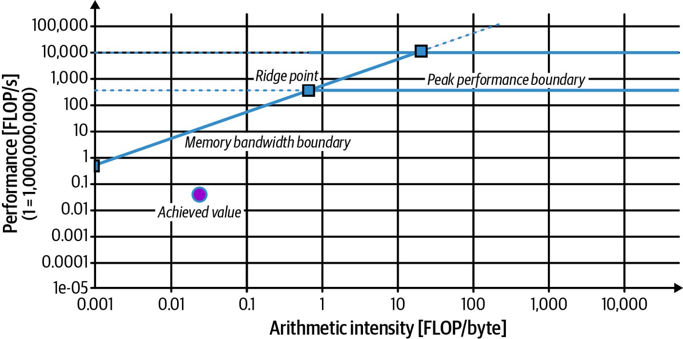
Figure 8-3. Chrome tracing visualization generated by the PyTorch profiler
PyTorch profiler allows you to identify bottleneck operations in your model code directly. For example, you can profile a training loop with torch.profiler.pro file(..., with_flops=True, profile_memory=True) to record memory usage and to estimate FLOPs for supported operators such as matrix multiplication. (Note: These are formula-based estimates at the operator level rather than per-kernel hard‐ ware counters.) Such integration makes it easier to bridge the gap between PyTorch model code and low-level CUDA performance analysis. Modern versions of Nsight Systems can collect Python backtrace sampling and also provide a PyTorch-focused mode, which supports Python call-stack sampling and a PyTorch domain for more correlated tracing.” This helps correlate framework activity with the system timeline. Nsight Compute correlates to CUDA C or C++ source and PTX or SASS. You can compile device code with -lineinfo to enable source line mapping. To correlate model code with kernels, use NVTX ranges from Python using torch.cuda.nvtx. In addition, modern versions of Nsight Compute provide a source view, which includes instruction mix—as well as a throughput breakdown that helps pinpoint the source code lines impacted by stalls and throughput limitations.
                     The lack of capturing Python information traditionally discour‐
                     aged PyTorch developers from using Nsight Systems/Compute.
                     However, if you are using PyTorch/Python, it’s worth revisiting
                     these tools to provide a more holistic and correlated analysis with
                     the rest of the system.
292 | Chapter 8: Occupancy Tuning, Warp Efficiency, and Instruction-Level Parallelism
This section outlines a workflow for diagnosing GPU bottlenecks, including how to interpret key profiler metrics and what they imply about the bottleneck type. We will focus on Nsight Compute for deep-dive kernel analysis, including warp stalls and memory throughput—and Nsight Systems for high-level application profiling, including concurrency and CPU-GPU overlap.
Profiler-Guided Analysis The key is to use all of these insights to guide your next steps since different bottle‐ necks require different optimizations. For instance, you can take advantage of Nsight Compute’s guided analysis rules, which might flag “Memory Bound: L2 transactions per FLOP high” or “Compute Bound: issue stall reasons indicate pipe contention.” These rules are updated for each architecture, including Blackwell. They can quickly confirm whether a bottleneck is in memory throughput, instruction dispatch, latency hiding, etc. This can direct you to the most relevant metrics and improve your bottle‐ neck time-to-resolution.
               Nsight Systems and Nsight Compute are constantly updated to the
               latest GPU architectures to assist performance engineers in diag‐
               nosing and fixing performance issues when migrating workloads to
               newer GPU generations.
Analyzing Warp Stall Reasons with Nsight Compute As discussed in Chapter 6, NVIDIA GPUs execute warps, or groups of 32 threads, in SIMT fashion. If warps are frequently pausing instead of issuing instructions, the profiler categorizes the reasons why. One of the most insightful views in Nsight Compute is the Warp State Statistics breakdown for a kernel. This is sometimes called the warp stall reasons. By examining these stall reasons, you can often pinpoint the limiting factor. There are a few different types of warp stalls: memory-related, execution dependency, execution contention, and others like texture-cache-related stalls. Let’s take a look at each of these.
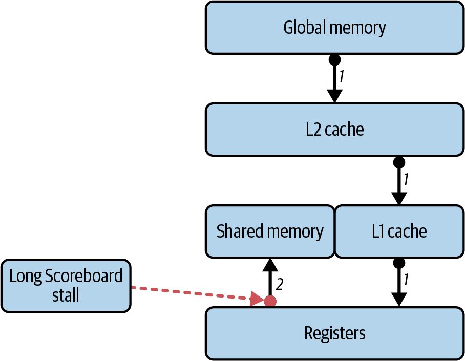
Memory-Related Stalls If a kernel is waiting on global memory loads, Nsight Compute reports a high per‐ centage of “Stall: Long Scoreboard” cycles. The scoreboard tracks each warp’s out‐ standing memory requests, so Long Scoreboard indicates warps frequently waiting on the high latency of global DRAM loads, as shown in Figure 8-4.
Analyzing Warp Stall Reasons with Nsight Compute | 293
Figure 8-4. Long Scoreboard stall caused by waiting on high-latency global memory accesses (e.g., waiting for data fetched from device memory into registers, or for spilled local memory to be written to/from device memory)
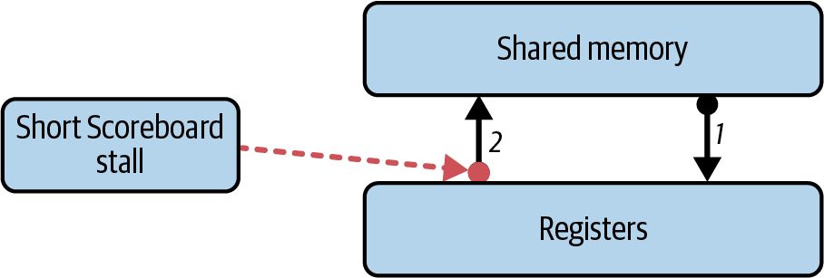
Similarly, a Short Scoreboard stall is caused by waiting on memory transfers between shared memory and the registers. This is shown in Figure 8-5.
Figure 8-5. Short Scoreboard stall caused by high-latency data transfers between shared memory and the registers
Similarly, metrics labeled “Stall: Memory Throttle” mean the load/store pipelines are saturated so that no additional memory requests can be issued because the hardware’s memory queues are full. “Stall: Not Selected” means that although warps are eligible to issue, they must wait for free memory transaction slots before they can proceed. Whenever these memory-related stall reasons dominate your stall profile, it is a clear sign the kernel is memory bound.
                    Use Nsight Compute’s source code view to highlight code impacted
                    by scoreboard dependencies and other hardware limitations (e.g.,
                    special function unit throughput, etc.).
294 | Chapter 8: Occupancy Tuning, Warp Efficiency, and Instruction-Level Parallelism
Execution-Dependency Stalls A high fraction of “Stall: Exec Dependency” means that warps are often waiting on the results of previous instructions. For instance, one instruction depends on the out‐ put of a prior instruction that has not yet completed. This is usually a sign of insuffi‐ cient instruction-level parallelism within each thread—or an ALU latency bottleneck. In a simple sequence of dependent arithmetic operations, later instructions must wait for earlier ones to finish. This causes the warp to go idle. If Exec Dependency stalls dominate, the kernel is likely latency bound waiting on compute. In other words, each thread’s instruction pipeline isn’t busy enough due to sequential dependencies.
Execution Unit Contention If you see significant “Stall: Compute Unit Busy”—or simply very high active utiliza‐ tion of the FP32 CUDA cores or Tensor Cores—the kernel is likely compute bound. In this case, the math units (FP32/FP64 ALUs, Tensor Cores, etc.) are saturated. Specifically, warps are ready to execute more instructions, but the execution units can’t service them any faster. This often manifests as near-peak “ALU pipe busy” met‐ rics and can correlate with high power usage. A related stall reason on some GPUs is “Stall: Math Pipe Throttle,” which means that warps are waiting because the math pipelines are fully occupied on every cycle.
Other Stall Reasons While the previous stall reasons are the most common culprits, there are many other less common stall categories, including instruction fetch stalls, texture unit stalls, syn‐ chronization stalls, etc. For instance, “Stall: Memory Dependency” is similar to Long Scoreboard in which an operation is waiting on a prior memory operation. “Stall: Texture Throttle” indicates a bottleneck in the texture caching subsystem. “No Eligible” or “Idle” indicates the warp scheduler had no warps ready to issue at a given cycle. This is often due to a prior synchronization—or simply not enough warps launched. In practice, you don’t need to memorize every stall reason. Instead, look at the largest portions of the stall breakdown. If memory-related stalls dominate, it’s memory bound. If execution dependency dominates, it’s latency bound on ALU. If there are almost no stalls and near 100% pipeline active, it’s likely compute bound. If warps are often “not selected” or idle, it could indicate insufficient parallel work or an occupancy issue. By examining the warp stall breakdown for your kernel, you can narrow down the bottleneck category.
Analyzing Warp Stall Reasons with Nsight Compute | 295
                     Nsight Compute provides these stall metrics per kernel launch.
                     Make sure to profile representative workloads. A tiny test kernel
                     might not exhibit the same stall profile as your real application.
                     Always collect data from realistic runs before drawing conclusions.
Table 8-1 shows a list of common warp stall reasons, their typical interpretation, and possible optimization approaches.
Table 8-1. Common warp stall reasons and optimization hints
Warp stall          Meaning/cause                                Potential optimizations
reason
Execution           Warp is stalled on a prior, dependent     Increase ILP (do independent work in the same thread).
dependency          instruction. This often indicates         Unroll loops or reorder instructions so that long-latency
                    insufficient instruction-level parallelismoperations (like multiplies or complex math) have other
                    (ILP) within the thread.                  work to overlap with. If ILP is maxed and still stalling, rely
                                                              on more warps (occupancy) to hide the latency.
Memory             The warp is waiting on memory loads        Hide memory latency by having more warps ready to run, or
dependency         (“long-latency”) to complete before it can higher occupancy, so that other warps can run while this
(Long Scoreboard proceed. No other work in the warp can       warp waits. Or use asynchronous memory prefetch to copy
stall)             proceed until data arrives.                data to shared memory, then continue computing. This will
                                                              overlap memory operations with computation. To minimize
                                                              latency, make sure that memory accesses are efficient, use
                                                              proper coalescing, and exploit proper cache hierarchies. On
                                                              modern GPUs, you should use the Tensor Memory
                                                              Accelerator (TMA) for bulk multidimensional copies so
                                                              memory movement overlaps compute with low thread
                                                              overhead.
Synchronization Warp is waiting at a __sync                   Reduce unnecessary synchronization. Reexamine the
(barrier)          threads() or other synchronization,        algorithm for ways to combine phases or use fine-grained
                   idle until all threads reach the barrier.  sync. Ensure work is evenly distributed so warps reach
                   Often indicates either frequent            barriers at roughly the same time. In some cases, use newer
                   synchronization or load imbalance (some sync primitives (e.g., warp-level sync or cluster sync) to limit
                   warps arrive earlier and wait).            scope of synchronization.
Instruction fetch/ Warp is stalled waiting to fetch the next If instruction cache misses are an issue, consider reducing
issue              instruction (could be an instruction cache kernel size (split kernel or avoid excessive unrolling that
                   miss or pipeline issue) or not issued      blows up code size). If pipeline issue (one type of instruction
                   because the required execution pipe was saturating a functional unit), try to mix instruction types or
                   busy. This can happen with very large      again use ILP to utilize different pipelines.
                   kernels or under certain pipeline
                   contention scenarios.
296 | Chapter 8: Occupancy Tuning, Warp Efficiency, and Instruction-Level Parallelism
Warp stall     Meaning/cause                                   Potential optimizations
reason
Not selected   The warp is ready but was not selected to       Usually not a problem—it means the GPU had other work
(scheduler)    issue in that cycle (scheduler picked           to do and chose a different warp for that cycle. If you see a
               another warp). This typically means there       high percentage of “Not Selected,” it implies high occupancy
               were other warps available and this one         is doing its job (hiding latency). No action needed unless it
               simply waited its turn. It is not a             indicates an imbalance (one warp hogging the scheduler; in
               dependency stall. It usually indicates that     rare cases, you might use scheduler hints or yield).
               other ready warps were chosen to issue
               that cycle, which is expected at healthy
               occupancy.
By interpreting these stall reasons, you can decide which optimization to pursue. For example, high memory stall time means you should try to hide latency with more warps, better memory access patterns, or asynchronous prefetch. Seeing high execution dependency stalls suggests that you should increase ILP or rearrange code. Frequent barrier stalls mean you should likely rework synchroniza‐ tion. This profiling step guides you to the most effective optimizations rather than blindly tuning everything.
Inspecting Achieved Occupancy and GPU Utilization Another key metric reported by profilers is achieved occupancy, or the average frac‐ tion of hardware thread slots, warps, that were occupied on each SM during execu‐ tion. For example, if a GPU supports 64 warps per streaming multiprocessor (SM) and achieved occupancy is 30%, then on average 19 warps were active per SM. Low achieved occupancy often signals underutilization since you can’t hide enough latency with only a few active warps. On the other hand, if you’re running at nearmaximum occupancy, but still not seeing the expected performance benefits, other bottlenecks are likely the cause. These include memory bandwidth limitations, ineffi‐ cient instruction streams, and suboptimal memory-access patterns. In these nonideal cases, simply adding more threads won’t help. Instead, you should investigate to improve memory coalescing, increase arithmetic intensity, and opti‐ mize warp‐level efficiency. We’ll cover these techniques in the upcoming sections. Nsight Compute also reports occupancy limiters, including which resource is con‐ straining the theoretical occupancy. For example, “Limited by max registers per thread” means your kernel’s register usage is preventing more warps from being scheduled per SM. However, “Limited by shared memory per block” means the kernel’s shared memory allocation per block is the bottleneck for occupancy. And “Limited by thread count”
Inspecting Achieved Occupancy and GPU Utilization | 297
means the launch configuration itself, grid, or block size didn’t request enough threads to fill the GPU. Each of these limiters hints at different fixes, which we will discuss in more detail in the next section. For instance, if registers are the limiter, you might reduce register usage or use __launch_bounds__ to allow more blocks. If shared memory is the lim‐ iter, you can try to use smaller tiles and less shared memory per block. Beyond a certain point, increasing occupancy may not produce a speedup. Very low occupancy (e.g., 10%–20%) will hurt performance due to poor latency hiding. On the other hand, pushing occupancy to 100% isn’t always beneficial if other factors like memory bandwidth and instruction dependencies become the bottleneck. As such, you should examine hardware utilization beyond just occupancy. Nsight Compute reports metrics such as achieved memory bandwidth in GB/s, achieved FLOPS in TFLOPS, instructions per cycle (IPC), issue-slot utilization, and other resource utilization statistics. These numbers will show how close your kernel is to the GPU’s physical hardware limits. For example, if your kernel’s ALU utilization is low while its memory throughput is at 95% of peak, you are almost certainly memory-bandwidth bound. Conversely, if ALU utilization is near its maximum but memory throughput remains modest, the kernel is compute bound. In this case, you’ll gain speed only by increasing arithmetic throughput—typically by switching to lower-precision types (FP16, FP8, or FP4) and moving work onto the faster Tensor Cores of the GPUs. If both ALU utilization and memory throughput are low, your kernel may be experi‐ encing long-latency operations, synchronization overhead, or simply insufficient par‐ allel work. This could indicate low instruction-level parallelism (discussed in an upcoming section)—or that you haven’t launched enough threads to fully utilize the GPU. You can frame this analysis using the Roofline model, which plots a kernel’s FLOPS against its arithmetic intensity (FLOPS per byte of memory accessed). The roofline defines a compute roof (the maximum FLOPS the GPU can sustain) and a memory roof (the maximum memory bandwidth). If your kernel’s FLOP/byte ratio falls below the hardware’s compute-to-memory ratio, you are memory bound because you cannot supply data fast enough. If the ratio is high but actual FLOPS remains far below peak, the kernel may be latency bound or lacking sufficient ILP to saturate the compute units.
                     With each new GPU generation, memory bandwidth increases
                     modestly, but compute capacity grows much faster. As such, ker‐
                     nels tend to become more memory bound over time.
298 | Chapter 8: Occupancy Tuning, Warp Efficiency, and Instruction-Level Parallelism
In practice, always compare two key figures: your kernel’s memory throughput versus the hardware’s peak memory bandwidth—as well as your kernel’s compute through‐ put versus the hardware’s peak FLOPS. Those comparisons will tell you whether your next optimization should focus on memory access, compute work, or parallelism. Let’s look at each of these next.
Kernel Memory Throughput Versus Peak HBM Memory Bandwidth Nsight Compute reports how many GB/s your kernel achieves. If your kernel is show‐ ing near-peak memory bandwidth utilization, performing more computations won’t help. You would have to increase arithmetic intensity by reducing memory traffic per operation. You can increase arithmetic intensity by using reduced precision with Tensor Cores, hiding more latency with concurrency, and using kernel fusion, which we’ll cover in a bit. These techniques help reduce global memory traffic by decreasing the size of intermediate data that is being transferred. For instance, if a kernel hits ~80% or more of the GPU’s memory bandwidth, it’s likely memory bound since there is little headroom left. However, note that Blackwell GPUs have a relatively large 126 MB L2 cache. And their dual-die design uses a high-bandwidth 10 TB/s interconnect, NVIDIA HighBandwidth Interface (NV-HBI), so the two GPU dies behave as one for memory access. As such, many kernels that were previously memory bound on older GPUs might better utilize the cache with newer GPU generations. You can use Nsight Compute’s memory chart to see how much traffic goes to L2 ver‐ sus DRAM. A high L2 hit rate could alleviate global memory bottlenecks, which means the kernel might actually be compute-limited despite performing heavy mem‐ ory accesses. The on-chip cache is servicing a lot of the memory accesses.
               On Blackwell, you can control L2 data persistence to keep critical
               working sets resident.
Kernel Compute Throughput Versus Peak GPU FLOPS Low achieved FLOPS can be caused by low occupancy or instruction-level stalls. For example, if only 30% of warps are active on average—or if pipelines are often idle due to memory waits—the kernel will sit far below the compute roof.
Inspecting Achieved Occupancy and GPU Utilization | 299
You can use Nsight Compute’s Occupancy section and Source Counters to pinpoint these issues. Ensure the kernel launches enough threads to fill the GPU, up to the perSM resident warps limit for your device (e.g., 64 resident warps per SM.)
                     Only warps within the same SM must share resources—and they
                     can hide one another’s latency. Warps on different SMs have no
                     interaction. As such, achieved occupancy is measured per SM.
                     We’ll cover occupancy in a bit.
Additionally, examine instruction issue efficiency and throughput metrics. Blackwell scales to many SMs per device, so underutilization at the kernel level can translate to large aggregate losses. (Note: The dual-die packaging does not, by itself, increase the per-SM issue rate.) If the achieved FLOPS are moderate to high but memory throughput is low, the ker‐ nel might be mostly compute-focused but limited by instruction dependencies. You can confirm by checking the “Exec Dependency” stalls metric in Nsight Compute— and any other stall reasons. If compute throughput is near peak, then you are truly compute bound. In this case, you have already optimized the kernel’s memory access patterns—or you are already using lower-precision Tensor Cores to reach such high FLOPS. Prolonged near-peak compute utilization can sometimes invoke power management compute limiters on modern GPUs to keep them healthy. Be sure to take this into account when you’re profiling, benchmarking, and tuning. The easiest way to see if you’re being power-limited is to use the following to monitor the enforced power limit alongside any “HW Slowdown” flags in real time: nvidia-smi \ --query-gpu=\ power.draw,clocks.current.sm,clocks.current.memory,\ clocks_event_reasons.active \ --format=csv -l 1 This command prints a new line every 1 second with current power draw, graphics/ memory clocks, and throttle reasons. With this information you can pinpoint when the GPU hits its power cap and downclocks. You can also use NVIDIA’s Management Library (NVML) API, which provides pro‐ grammatic access to the CUDA C++ nvmlDeviceGetPowerUsage() and nvmlDevice GetEnforcedPowerLimit() APIs—as well as the equivalent NVML Python APIs. These are ideal for custom scripts or integration with monitoring systems. In short, use a combination of occupancy, warp stall reasons, memory throughput, and compute throughput metrics together to diagnose the bottleneck. Make sure you
300 | Chapter 8: Occupancy Tuning, Warp Efficiency, and Instruction-Level Parallelism
see high occupancy, high warp efficiency, and a balanced usage of execution units, including Tensor Cores.
Iteratively Profiling and Determining the Kernel Bottleneck GPUs can stall for four fundamentally different reasons: underutilization, latency bound, memory bound, and compute bound. These regimes are related, but it’s important to understand each of them independently in order to choose the right optimizations to pursue. Often, fixing one bottleneck will reveal another. Underutilization happens when you simply haven’t launched enough threads or work. In this case, both FLOPS and memory bandwidth stay low and the execution timeline has idle gaps. Once you increase parallelism, you will find your warps are now stalling and waiting on memory loads. Once you more fully utilize your GPU, you can now distinguish between latency bound and memory bound. A latency-bound kernel issues far fewer bytes/sec than the hardware can deliver because individual memory loads are stalling the warps. The fix is to increase memory-compute overlap by increasing occupancy, using more ILP, prefetching, and pipelining. A memory-bound kernel, in contrast, is saturating DRAM bandwidth, but your ALUs are sitting idle, not because of stalls but because there’s simply no more data you can fetch per second due to the memory pipe saturation. In this case, you must raise arithmetic intensity with tiling, fusing, exploiting caches (L1/texture), or reducing precision to reduce memory traffic. If neither of those fixes produces more speed, you’ve moved into compute-bound ter‐ ritory in which the GPU’s arithmetic pipes (e.g., ALUs and Tensor Cores) are the lim‐ iting factor. Here you can increase per-thread ILP by overlapping independent instructions with unrolling and software pipelining. On modern GPUs, unified cores cannot execute an INT32 and an FP32 instruction in the same clock. In other words, mixed INT32 and FP32 workloads do not execute both types from the same core in the same cycle. As such, the achievable issue rate depends on your instruction mix. As you optimize, you’ll often find yourself working through these regimes as follows: underutilized → latency bound → memory bound → compute bound. After each fix, you will likely hit a new bottleneck and apply the corresponding strategy. When opti‐ mizing GPU code, you should follow a structured approach as described here. First, you should profile. Next, you can identify the bottleneck. You can use Nsight Compute for kernel-level metrics (e.g., warp stalls, achieved occupancy, memory ver‐ sus compute utilization) and Nsight Systems for application-level timelines (e.g., con‐ currency, idle gaps).
Inspecting Achieved Occupancy and GPU Utilization | 301
Once you identify the bottlenecks, you can determine if the kernel is memory bound, compute bound, latency bound, or simply underutilizing the GPU. The GPU is underutilized when it is not issuing enough work. Table 8-2 summarizes these four regimes, including common profiling indicators and remedies.
Table 8-2. Memory bound versus latency bound versus compute bound versus underutilizing
the GPU
Limiting factor   Description                                  Profiler indicators         Remedies
Memory bound      You’re moving as much data as you can        High memory-bandwidth       Increase arithmetic intensity (e.g.,
                  —close to peak DRAM bandwidth—but            utilization is near peak,   tiling, fusion) and improve
                  you don’t have enough work per byte to       low FLOPS.                  coalescing and caching.
                  fully utilize the ALUs.
Compute bound     You’ve hidden memory latency and are         High FLOPS are              Exploit more ILP (e.g., dual-issue,
                  no longer saturating memory                  approaching GPU peak,       loop unroll), use specialized units
                  bandwidth. Now the ALUs (e.g., CUDA          low memory utilization.     (e.g., FP16/FP8/FP4/Tensor
                  cores and Tensor Cores) are the                                          Cores), reduce dependencies, fuse
                  bottleneck.                                                              work, leverage lower precision or
                                                                                           sparsity.
Latency bound     You’re not sustaining enough concurrent      Low achieved bandwidth      Raise occupancy, add ILP (e.g.,
                  work to hide individual load/store           well below peak, high       unroll, multiple accumulators),
                  latencies, so warps stall waiting on data.   “stall-on-scoreboard” or    intra-kernel pipelining, and
                                                               “not selected”              software prefetch.
                                                               percentages.
Underutilizing    You’re not fully occupying SMs or            Low occupancy and low       Increase problem size or batch
the GPU           launching enough work—both memory            achieved bandwidth, low     work, launch more threads/
                  and compute resources remain idle.           FLOPS, timeline shows       blocks, fuse tasks, use persistent
                                                               gaps or sparse kernel       kernels (Chapter 10) or streams
                                                               activity.                   (Chapter 11).
A memory-bound kernel is one where performance is limited by memory throughput—specifically, if the GPU’s global memory is unable to feed data to the compute units fast enough. In this case, your kernel’s achieved FLOPS will sit near the roofline set by memory bandwidth. This happens if you have plenty of threads but can’t move data any faster. As such, you’re up against the memory-bandwidth ceiling. Conversely, a compute-bound kernel saturates the GPU’s arithmetic units (ALU FP32 CUDA cores or reduced-precision Tensor Cores). This is noticeable if the kernel is approaching the peak FLOPS roofline for the cores. Profiling metrics like achieved occupancy, memory utilization, and execution dependency stalls can help confirm this classification. When a kernel is latency bound, on the other hand, each thread spends a large frac‐ tion of its time waiting on individual memory loads instead of doing useful work. In practical terms, this means that when a warp issues a global‐memory load to fetch A[idx], for instance, all 32 threads in that warp will stall until that fetch completes. If
302 | Chapter 8: Occupancy Tuning, Warp Efficiency, and Instruction-Level Parallelism
the code immediately issues another dependent load or computation, the warp simply sits idle for hundreds of cycles on each load. The GPU’s warp scheduler may switch to other warps when it is latency bound, but if every warp is structured the same way (e.g., one load → wait → compute → write), there is rarely any other work to fill in those idle cycles. As such, the kernel never has enough independent operations in flight to hide the latency of a long‐latency DRAM access. To break out of the latency‐bound situation, you need to give the GPU multiple oper‐ ations to overlap. One approach is to increase occupancy by launching more threads and warps. This way, when one warp stalls on its load, another warp is ready to run. Equally important, though, is increasing each warp’s ILP. We’ll cover ILP in more detail later in this chapter. At a high level, if each thread issues two or more inde‐ pendent loads back‐to‐back by loading A[idx] and B[idx] before doing any arith‐ metic, the GPU can start overlapping those loads in hardware. In this case, while the first load waits for DRAM, load two (and three and four, etc.) can already be in flight. As soon as any of these loads return, the dependent arith‐ metic can execute. This will further overlap with the remaining pending loads.
                You can also increase ILP by unrolling a small loop so that multiple
                values are fetched before any computation. More on this later.
By increasing ILP, each thread and warp always has enough work in flight so that the DRAM latency is masked by other outstanding operations. The net effect is to trans‐ form a latency‐bound kernel into one that keeps the SM’s pipelines busy. This will increase throughput and overall kernel performance. When the GPU is underutilized, you’re not launching enough work to keep SMs and memory pipelines busy, so many resources remain idle. In this case, it will help to increase the amount of work by increasing the batch size or launching more threads.
Optimizing the Kernel In practice, performance tuning should follow a clear, step‐by‐step workflow. First, identify which regime your kernel occupies: memory bound, latency bound, compute bound, or underutilized. Next, apply the corresponding optimizations. If your kernel is memory bound, concentrate on reducing and hiding memory traffic. You can do this by improving coalescing, raising occupancy, increasing ILP, and introducing data reuse through caching or tiling.
Inspecting Achieved Occupancy and GPU Utilization | 303
When the kernel is latency bound, meaning individual load or instruction latencies
dominate, make sure there is enough independent work in flight. You can do this by
issuing multiple nondependent loads/operations per thread or increasing overall
occupancy so the scheduler always has ready warps to run.
If the kernel is compute‐bound (i.e., the ALUs or Tensor Cores are saturated while
memory is idle), shifting to lower‐precision arithmetic (FP16/FP8/FP4), offloading
work onto Tensor Cores, or fusing more operations together can raise arithmetic
throughput. Finally, if the GPU appears underutilized with low occupancy and fre‐
quent idle cycles, simply launching more threads or blocks (so that all SMs have
work) is often enough to get the hardware busy before applying deeper optimizations.
Here is a list of high-level optimization techniques that help you treat GPU perfor‐
mance tuning as a scientific process. We’ll dive into these over the next few chapters,
but they should each include identifying the limiting factor, applying the appropriate
optimization, and measuring the outcome:
Convert memory-bound workloads to compute bound
   If memory bound (low arithmetic intensity), increase data reuse and work per
   launch as follows: apply tiling to use fast shared memory and reduce redundant
   accesses, fuse kernels to avoid unnecessary memory round trips, ensure memory
   accesses are optimized (coalesced, avoiding bank conflicts as per Chapter 6), and
   consider using compression or lower precision to move less data.
Further optimize compute-bound workloads
    If compute bound (e.g., high utilization of ALUs but not hitting peak due to
    dependencies), increase effective instruction throughput as follows: use ILP tech‐
    niques (e.g., unroll loops, multiple accumulators to overlap independent ops),
    check for branch divergence (see Chapter 6) and try to reorganize work to reduce
    it since divergence wastes ALU cycles, and move to Tensor Cores and lower pre‐
    cision to raise the compute ceiling. If the kernel is at compute roof, see if reduc‐
    ing precision (FP32 → FP16 → FP8 → FP4) can give further speedups.
Increase parallelism for latency-bound workloads
    If latency bound (e.g., frequent warp stalls and not enough parallelism to hide
    latency), increase concurrency at various levels as follows: launch more threads/
    blocks if possible until latency is hidden, ensure registers/shared memory are not
    overly limiting occupancy (e.g., occupancy tuning and balancing resource usage),
    overlap memory and compute within each thread/warp using async copies (e.g.,
    intra-kernel pipelining), and use multiple streams to overlap independent tasks
    or overlap copies with compute (e.g., inter-kernel concurrency described in
    Chapter 11). If launch overhead is an issue (e.g., many tiny kernels), consider
    merging them with cooperative groups or simply combining their code (e.g., ker‐
    nel fusion).
304 | Chapter 8: Occupancy Tuning, Warp Efficiency, and Instruction-Level Parallelism
Increase GPU utilization
    If the GPU is underutilized (e.g., low SM Active, low occupancy), ensure you
    launch enough work to use all SMs. Specifically, make sure your kernel is launch‐
    ing with a grid size large enough to fully utilize the GPU. A common mistake is
    launching as many threads as elements but forgetting that each thread does only
    a little bit of work. Sometimes you need multiple passes or more threads per
    element.
Reduce synchronizations and host-side (CPU) stalls
   You should remove any unnecessary cudaDeviceSynchronize() or host-side waits
   that stall the GPU. If the workload is inherently small, consider batching it with
   other work or running multiple instances concurrently (e.g., CUDA streams).
   You can also use CUDA Graphs (see Chapter 12) to predefine and efficiently
   launch an execution graph of many small kernels.
Leverage specialized hardware and reduced/mixed precision
    Blackwell Tensor Cores expose fifth-generation MMA instructions in PTX as
    tcgen05.mma and associated loads/stores (e.g., tcgen05.ld and tcgen05.st).
    Tensor Cores accelerate microscaling formats including MXFP8, MXFP4 (OCP
    MX formats), and NVIDIA’s NVFP4 format. They also support block-scaled mat‐
    muls (K-grouped) that libraries select automatically when scale metadata is
    present. TMEM and TMA underpin these high-throughput data paths. We’ll dis‐
    cuss these techniques in more detail later in this chapter and in Chapter 9.
Verify and iterate
    After each optimization, reprofile. Confirm the targeted stall or metric improved
    (e.g., memory stalls reduced after tiling, achieved occupancy went up after tuning
    block size, “SM Throughput %” increased after using CUDA streams, etc.). Also
    watch total runtime improvement. Sometimes one bottleneck masks another;
    you might fix memory bandwidth only to become compute bound next (which is
    fine—then address that if needed).
Maintain correctness and acceptable accuracy
   When using lower-precision or new parallel strategies, test with assertions or
   comparisons to reference results. Ensure the speedup doesn’t come at the cost of
   accuracy unless that’s acceptable for the application. Typically, techniques like
   FP16 or even FP8 are carefully validated to have negligible accuracy impact on AI
   models.
Inspecting Achieved Occupancy and GPU Utilization | 305
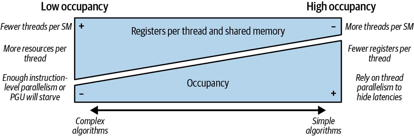
Tuning Occupancy Remember from Chapter 6 that occupancy is the ratio of active warps on the SM to the maximum number of warps that could be active on the SM. Low occupancy (< 50%) means that, on average, half of the possible warps were active. This might indicate that your kernel is limited by resources such as registers or shared memory per thread block—rather than just available parallelism. Occupancy is the measure of how many threads, or warps, are active on an SM rela‐ tive to the hardware’s maximum capacity. Higher occupancy, or more warps in flight, allows the GPU to better hide latency. This is because when one warp stalls waiting on a memory load, for instance, the scheduler can quickly switch to run another warp. More warps per SM generally means the GPU’s pipelines stay busier, and fewer cycles are wasted waiting on memory. Occupancy tuning is the practice of adjusting your kernel launch parameters and resource usage (e.g., registers and shared memory) to maximize useful parallelism on each SM, as shown in Figure 8-6.
Figure 8-6. Tuning occupancy by balancing resource usage (e.g., registers per thread and shared memory) with parallelism (e.g., number of threads and warps)
Remember that the goal of occupancy tuning is to keep enough warps active to fully utilize the SM’s pipelines and hide long‐latency operations. In an ideal case, you would achieve 100% occupancy, filling all available warp slots. For instance, there are 64 warp slots, or 2,048 threads, available in each Blackwell B200 (compute capability 10.0) SM.
306 | Chapter 8: Occupancy Tuning, Warp Efficiency, and Instruction-Level Parallelism
               This per-SM limit of 64 warps has remained the same for modern
               datacenter GPU architectures like Ampere, Hopper, and Blackwell—
               even as the overall GPU core counts have increased. The hardware-
               performance improvements come from more SMs, larger caches,
               multidie, etc. You can use Nsight Compute’s Occupancy analysis to
               confirm the exact limits on your target device. Interestingly, the
               NVIDIA RTX PRO 6000 and Spark DGX (GB10 superchip) support
               a higher compute capability (12.x), but only allow 48 warps (1,536
               threads) per SM.
Many real‐world kernels still perform well at lower occupancy—especially if their memory or arithmetic latencies are already small. Or if they leverage high‐ throughput units like Tensor Cores that keep the pipelines busy without needing as many active warps. For instance, a compute-bound kernel might achieve peak performance with only 50% occupancy because each warp is doing lots of work without waiting. In contrast, a memory-bound kernel often benefits from high occupancy since some warps can run on the SM since other warps are stalled waiting for memory transfers.
Find the Right Occupancy for Your Workload In practice, effective occupancy tuning often produces diminishing returns after a certain point. If a kernel is severely memory bound, for instance, going from 10% to 50% achieved occupancy might give a huge boost because now you have enough warps to cover latency. But going from 50% to 100% might give only a small further gain since other factors start to dominate, such as cache misses, memory bandwidth saturation, etc. Profiling helps determine the optimal occupancy. For example, you can evaluate profile metrics such as eligible warps per cycle and active warps per scheduler. These give insight into how many warps are ready to issue versus how many the hardware could handle. Eligible warps per cycle reports the average number of warps that are in a “ready-torun” state each cycle and have no outstanding data or dependency stalls. Active warps per scheduler, often equal to the number of schedulers on the SM, is the maximum number of warps that could issue an instruction per cycle. If eligible warps per cycle is lower than active warps per scheduler, the GPU often runs out of ready warps. In this case, when one warp stalls on memory or a longlatency instruction, there isn’t another ready warp to switch to. This indicates you need more concurrency in the form of higher occupancy or ILP to hide the latency. In contrast, if eligible warps per cycle meets or exceeds the scheduler limit but your kernel still runs slowly, it means you have enough warps ready, but they cannot issue because of other stalls such as memory-bandwidth saturation or execution
Tuning Occupancy | 307
dependencies. In this case, it’s best to focus on hiding memory latency through better coalescing and asynchronous copies—or increasing ILP by unrolling independent work. This is a better approach than simply adding more threads. And if you raise occupancy and see the “Stall: Not Selected” or idle percentages drop, and memory pipes are busy more often, you’ve successfully improved occupancy. If occupancy is high but Long Scoreboard is still dominant, you might need other tech‐ niques like improving memory access patterns or overlapping computation. In practice, once you reach a moderate occupancy (e.g., 60%–70%), the returns will start to diminish. As such, it’s often more effective to pursue better memory locality, higher ILP, and the use of on-chip memory like shared memory and registers to cache data. While maximizing occupancy ensures that many warps are available to run, those warps might still be idle if waiting on memory or if executing divergent code. There‐ fore, after achieving a reasonable occupancy (e.g., 50%–70%), focus on warp effi‐ ciency and latency-hiding rather than obsessing over 100% occupancy.
                    Occupancy is a means to an end (hiding latency), not the end goal
                    itself. Once you have enough warps to keep the GPU busy, other
                    optimizations will give better returns.
Techniques for Occupancy Tuning
There are a few straightforward steps to improve occupancy when profiling suggests
that it’s the limiting factor: increase parallelism by launching more threads, adjust the
block size, reduce per-thread resource usage, and use __launch_bounds__ or the
occupancy API. Let’s discuss each of these here:
Increase parallelism (launch more threads)
    The simplest way to improve occupancy is to launch more work if your current
    kernel launch isn’t already using all SMs. For instance, if you launch only 20
    warps per SM and the GPU can support 64, increasing your grid size or threads
    per block can raise occupancy (assuming enough data to process).
      Be sure to utilize all SMs by launching at least as many blocks as SMs—and often
      many more since blocks execute in parallel on each SM. If your GPU shows low
      “SM Active Cycles” because not all SMs have work, scale up the workload or
      batch size. However, simply using more threads isn’t enough—especially if each
      thread uses a lot of resources such as registers and shared memory.
308 | Chapter 8: Occupancy Tuning, Warp Efficiency, and Instruction-Level Parallelism
Adjust block size
    Sometimes the number of threads per block, or thread-block size, can limit occu‐
    pancy. Very large thread blocks (e.g., 1,024 threads) might use so many registers
    or so much shared memory that only one block can fit on an SM at a time. This
    results in low occupancy. In contrast, using moderately sized blocks (e.g., 128–
    256 threads) allows multiple blocks to reside concurrently on one SM, which
    increases the total number of possible active warps.
    The optimal block size can vary by kernel. The key is to balance block size
    against resource usage. Smaller blocks use fewer resources individually and
    therefore allow more blocks in parallel.
    You can use the built-in Nsight Compute Occupancy Calculator and the CUDA
    Occupancy API to experiment with different launch configurations to help find a
    sweet spot that maximizes occupancy without incurring other overheads.
    The Occupancy Calculator suggests configurations for maximum theoretical
    occupancy. However, the best performance in practice might come from an occu‐
    pancy that is slightly less than this theoretical maximum.
                    Always validate the Occupancy Calculator’s suggested best
                    BlockSize with actual timing experiments, as sometimes a
                    configuration with a bit lower occupancy produces higher
                    throughput due to less register spilling or better memory
                    coalescing.
Reduce per‐thread register and shared-memory usage
   Each thread consumes registers—and likely shared memory. If a kernel uses too
   many registers or shared memory per thread, the compiler must reduce how
   many threads or warps can be active on an SM. Otherwise, it will exceed the SM’s
   total register file or shared-memory allocation.
    To address register usage, you can refactor your code to use fewer live variables,
    and therefore fewer registers, to free up register capacity. This allows more warps
    to be resident simultaneously. Similarly, you can pass -maxrregcount=<N> to the
    compiler to cap the number of registers allocated per thread.
    When you cap the number of registers per thread, the compiler is forced to fit
    each thread into fewer registers. This allows the hardware to schedule additional
    warps on the SM—and therefore raises occupancy.
    Of course, if you cap registers too aggressively, the compiler will spill excess vari‐
    ables into local memory, which will hurt performance. As such, you should find
    the smallest register limit that maximizes occupancy without excessive spilling.
Tuning Occupancy | 309
      Similarly, if each block uses a large amount of shared memory such as a large tile,
      shared memory will limit how many blocks fit on an SM. By optimizing the
      shared memory footprint, storing only what’s needed, and using on-chip caches
      when possible, you can free up capacity for additional blocks. Essentially, you can
      increase occupancy by using leaner resources per thread/block.
      Be mindful, however, that reducing registers or shared memory might degrade
      single-thread performance if taken too far. It’s a trade-off. The profiler’s Occu‐
      pancy limiter readout will tell you if registers or shared memory are the bottle‐
      neck. This will help guide your optimization efforts.
      For instance, on Blackwell, you may see “Limited by max registers per thread” if
      you aggressively unroll loops. In this case, consider using fewer unrolled itera‐
      tions or splitting the work. This is because Blackwell has a 255 register-per-
      thread limit. The Occupancy report helps quantify these trade-offs.
Use __launch_bounds__
    In some scenarios, you might deliberately limit occupancy or guide the compiler
    to optimize for a specific occupancy. CUDA allows you to set launch bounds in
    the kernel code using the __launch_bounds__ annotation. This gives a hint to the
    compiler of the kernel’s intended usage pattern and launch configuration.
      If you profile and find that performance peaks at an occupancy around 50%
      rather than 100%, it often means that each thread is using a lot of registers or
      shared memory. This will further limit occupancy. In such cases, you can guide
      the compiler using __launch_bounds__.
      For example, you can use __launch_bounds__ to limit the threads-per-block and
      specify a minimum blocks-per-SM to allow more warps to reside on the SM.
      Essentially, you’re telling the compiler to trade some per-thread register/shared-
      memory resource usage for a higher warp count.
      This will improve throughput when your kernel is latency bound because more
      warps will hide memory latency and dependency stalls. This is opposed to a
      purely compute-bound kernel, which wouldn’t see the same gain from this type
      of optimization.
Use the CUDA Occupancy API
    In addition to the __launch_bounds__ annotation, CUDA’s Occupancy API func‐
    tions (e.g., cudaOccupancyMaxPotentialBlockSize() and cudaOccupancyMax
    ActiveBlocksPerMultiprocessor()) let you determine, at runtime, the block
    size that produces the highest occupancy given your kernel’s actual register and
    shared‐memory demands.
      These functions provide recommended values for threads per block and the
      number of blocks per SM. This way, you don’t have to guess which configuration
310 | Chapter 8: Occupancy Tuning, Warp Efficiency, and Instruction-Level Parallelism
    is most efficient. In practice, you might use the Occupancy API to find a candi‐
    date block size and then fine‐tune it with a __launch_bounds__ hint to lock in a
    specific occupancy level.
               Another approach is to use CUDA Graphs to launch predefined
               workloads efficiently once you’ve determined the optimal configu‐
               ration. While not directly changing occupancy, CUDA Graphs can
               reduce per-launch overhead, which is beneficial for occupancy
               when you increase the number of blocks. We’ll cover CUDA
               Graphs in Chapter 12 and PyTorch’s use of CUDA Graphs in Chap‐
               ters 13 and 14, but it’s worth mentioning them in this context.
               In short, it’s recommended to use a multiphased approach by
               profiling your system to discover the ideal occupancy range—and
               then using compiler and runtime hints to achieve the ideal occu‐
               pancy. The goal is to size your thread blocks efficiently to keep
               enough warps in flight without over allocating scarce on‐chip
               resources like registers and shared memory. Next, let’s take a closer
               look at tuning occupancy with __launch_bounds__, the Occupancy
               API, and PyTorch.
Compiler Hints to Optimize Occupancy We can guide the compiler to optimize for occupancy by using CUDA’s __launch_bounds__ kernel annotation. This annotation lets us specify two parame‐ ters for a kernel: the maximum number of threads per block that we want to launch (e.g., 256) and the minimum number of thread blocks we want to keep resident on each SM (e.g., 4), as shown here: __global__ __launch_bounds__(256, 8) void myKernel(...) { /* ... */ }
Here, we promise never to launch myKernel with more than 256 threads per block. And we request that the GPU tries to keep at least 8 blocks active per SM. These hints influence the compiler’s register allocation and inlining decisions. Specifically, __launch_bounds__ will limit each thread’s register usage such that up to 256 threads can fit in one block—and at least 8 blocks can be active per SM. This is a total of 2,048 threads active per SM (8 blocks × 256 threads per block = 2,048 threads). This fills the thread slots for devices like the B200 with a 2,048-thread perSM limit (e.g., Blackwell). In practice, __launch_bounds__ can cause the compiler to cap per-thread register usage and restrict unrolling/inlining. This avoids spilling and allows higher occupancy. As such, we are effectively trading a bit of per-thread per‐ formance (e.g., not using every last register or unrolling to the max) in exchange for steadier warp throughput by keeping more warps in flight.
Tuning Occupancy | 311
                     Increased occupancy must be balanced with increased per-thread
                     resources. You want to avoid register spilling by forcing too many
                     threads. This causes slow memory access because they run out of
                     registers and spill to local memory (backed by global HBM.) Find‐
                     ing the sweet spot often requires experimentation. Nsight Com‐
                     pute’s “Registers per Thread” and “Occupancy” metrics can guide
                     you here.
Determine Optimal Launch Configuration with the Occupancy API You can determine an optimal launch configuration at runtime using the CUDA Occupancy API, including cudaOccupancyMaxActiveBlocks PerMultiprocessor() and cudaOccupancyMaxPotentialBlockSize(). For instance, cudaOccupancyMax PotentialBlockSize() will calculate the block size that produces the optimal occu‐ pancy for a given kernel, considering its register and shared memory usage as shown here: int minGridSize = 0, bestBlockSize = 0;
      cudaOccupancyMaxPotentialBlockSize(
          &minGridSize, &bestBlockSize,
          myKernel,
          /* dynamicSmemBytes = */ 0,
          /* blockSizeLimit = */ 0 );
// bestBlockSize contains number of threads per block that maximizes occupancy myKernel<<<minGridSize, bestBlockSize>>>(...); This API computes how many threads per block would likely maximize occupancy given the kernel’s resource usage. We can then use the suggested bestBlockSize and minGridSize for our kernel launch. In practice, the compiler’s heuristics are usually pretty good. But using __launch_bounds__ and the occupancy API can give you explicit control when needed. Use them when you know your kernel can trade some per-thread resource usage for more active warps. This helps prevent underoccupying SMs due to heavy threads.
Tuning Occupancy with PyTorch For PyTorch users writing high-level code, you don’t usually manage occupancy directly—PyTorch’s CUDA kernels and libraries handle launch parameters under the hood. Operations like matrix multiplies, convolutions, etc., are already tuned to use the GPU effectively. However, understanding occupancy can still be valuable. If you write custom CUDA kernels as PyTorch extensions, the same principles apply: launch enough threads/
312 | Chapter 8: Occupancy Tuning, Warp Efficiency, and Instruction-Level Parallelism
blocks to utilize the GPU, choose reasonable block sizes, and avoid using excessive registers or shared memory per thread if it limits occupancy. Even at the Python level, there are a few things to be mindful of. If you are using PyTorch and notice that your GPU is underutilized (e.g., in a profiling trace you see only a small fraction of SMs active), it could be because of very small tensor opera‐ tions that don’t launch many threads. Extremely small workloads might not scale well to a large GPU. In such cases, try batching or combining operations so that each launch does more work. PyTorch’s graph compiler can fuse certain operations using torch.compile. This increases the work per kernel launch—and therefore improves occupancy and efficiency.
                Under the hood, torch.compile generates fused GPU kernels. It
                does this by merging many small operations into one larger kernel.
                Whenever possible, leverage the PyTorch compiler, as it can
                achieve the efficiency of a manually written CUDA kernel in some
                cases. Prefer torch.compile(mode="max-autotune") for long-
                running training/inference on stable shapes, or mode="reduce-
                overhead" for small-batch, graph-friendly loops. Both enable
                CUDA Graphs when profitable. You can also use mode="max-
                autotune-no-cudagraphs" if graphs are undesirable. We dive deep
                into the PyTorch compiler and its different mode options in Chap‐
                ters 13 and 14.
It’s also worth noting that PyTorch’s built-in kernels often use best practices internally. For example, reduction operations and elementwise operations in PyTorch are imple‐ mented with launch configurators that pick an optimal block size and number of blocks based on the device and tensor size. If you ever dig into PyTorch’s C++ CUDA code, you’ll see logic to cap block sizes and to launch multiple blocks per SM for certain algorithms. This is essentially automated occupancy tuning. To reduce optimizer overhead, enable fused implementations where available. For instance, use torch.optim.AdamW(..., fused=True) and pair with automatic mixed-precision (AMP). The takeaway for PyTorch users is to prefer high-level libraries and operations that are already optimized. This is in preference to writing custom kernels. If you do need custom kernels, apply the same occupancy principles that we discussed. Now that we see how to keep the GPU busy with enough threads, we next turn to making each warp more efficient. High occupancy means little if each warp is wasting cycles. This leads us to our discussion on warp-level efficiency optimizations, includ‐ ing warp divergence and intrawarp thread cooperation.
Tuning Occupancy | 313
Improving Warp Execution Efficiency (Warp Divergence) Even with plenty of warps available, thanks to good occupancy, each warp’s internal efficiency matters. Warp execution efficiency measures the fraction of warp lanes that are active on average. Warp-level inefficiencies arise when threads within a warp do not all do the same work, called warp divergence. Another cause is if the threads are waiting on data loads. Specifically, a low warp execution efficiency value typically shows a high divergent branch count, low predicate efficiency, and possibly a high number of memoryrelated stalls. This means that the warp threads are idle due to branching divergence caused by if/else statements in the kernel or by data-dependencies. In this case, you should try to restructure your code to avoid the inefficiencies. To improve warp execution efficiency, you should try to improve memory coalescing, minimize thread divergence, and use warp-level intrinsics for optimal intrawarp (thread-level) communication. These techniques often produce modest speedups (say, 5%–30%) compared to higher-level algorithmic changes, but they can be crucial in highly optimized code where every cycle counts. They also complement other optimizations in that, after you’ve optimized occupancy and improved memory access, you can still squeeze out extra performance by ensuring each warp executes as efficiently as possible.
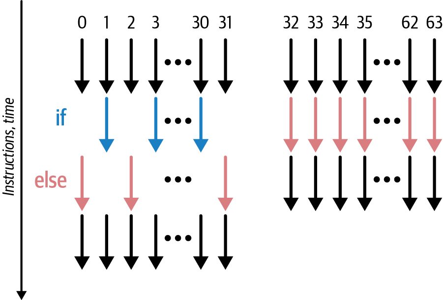
Causes of Warp Divergence As mentioned in Chapter 7, warp divergence, or branch divergence, occurs when threads in the same warp take different control-flow paths. For example, consider an if/else inside a kernel where some threads in a warp execute the if clause and oth‐ ers execute the else. In SIMT execution, the warp must execute both paths serially: first, all threads that take the if branch execute while the others in that warp are masked off (idle). Then the threads that took else execute while the first group idles, as shown in Figure 8-7. During the divergent sections, effectively only half, or some fraction, of the warp is doing useful work. This reduces overall throughput. In the case of a 50/50 split between if and else, the warp’s active utilization drops to 50% for that portion of code. If the split is 1 thread versus 31 threads, then 31/32 threads will be idle in one of the subbranches.
314 | Chapter 8: Occupancy Tuning, Warp Efficiency, and Instruction-Level Parallelism
Figure 8-7. Divergent versus nondivergent warp execution
                If your kernel contains multiple divergence points or if each diver‐
                gent branch carries heavier work, removing those branches can
                compound these gains. In the ideal case (e.g., a 50/50 split branch),
                removing that divergent branch can nearly double throughput up
                to ~2× speedup. Eliminating multiple heavy divergence paths can
                compound these gains.
The overall effect is that warp divergence causes some GPU cores to sit idle. This increases the total instruction count since each branch path is executed serially by dif‐ ferent subsets of threads. Therefore, minimizing intrawarp divergence is a key to warp-level efficiency.
Techniques to Avoid Warp Divergence There are various best practices to minimize warp divergence, including restructur‐ ing conditions and separating branches into multiple kernels.
                Warp divergence only affects threads within a warp. Threads in dif‐
                ferent warps do not cause each other to stall.
Improving Warp Execution Efficiency (Warp Divergence) | 315
Additionally, you can use warp-unanimous branches, warp-vote intrinsics, and predi‐
cation. Let’s discuss each of these:
Restructure conditions
    Wherever possible, organize your computations so that threads in the same warp
    follow the same execution path. This might involve moving a divergent condition
    to a higher level outside of the inner loops—or into a separate kernel launch. You
    could also sort or group your data so that each warp handles more homogeneous
    cases.
      For instance, if you have an array of values and you want to process negative val‐
      ues differently from nonnegative ones, a naive approach might put an if(x<0)
      inside the kernel that diverges per element. A smarter approach is to partition the
      data such that one kernel handles all negatives and another kernel handles non‐
      negatives. By aligning data with warps, you reduce the chance that a single warp
      has to split its execution.
Separate into multiple kernels
    Another approach is to separate the work into multiple kernel launches such that
    one kernel handles the if case and another handles the else case. You can use a
    prefix sum or compaction to distribute threads to the different kernels. This
    avoids divergence at the cost of launching more kernels and adding logic to dis‐
    tribute data between the kernels. This might be worth it if divergence is a big
    issue and the divergent sections are large enough in instruction count.
Rewrite conditions to be warp-unanimous
   In some cases, you can rewrite a condition to be warp-unanimous. This means
   that either all 32 threads in a warp satisfy the condition or none do. A common
   trick is to use the warp index in the condition statement. For instance, you first
   compute a warp ID as int warpId = threadIdx.x / 32;. Then half of your
   warps do task A and the other half do task B. For this, you write: if (warpId % 2
   == 0) { /* Task A */ } else { /* Task B */ }.
      In this case, all threads in a given warp either go into task A or task B together,
      and there’s no warp divergence since one warp executes one branch while
      another warp executes the other branch. But within a single warp, all threads
      agree on the branch to execute.
      The slight overhead is that every warp still evaluates the branch condition, but
      since they all agree on it, each warp executes only one of the branches. This tech‐
      nique essentially trades some flexibility—since you’re constraining how work is
      divided—to gain warp coherence.
316 | Chapter 8: Occupancy Tuning, Warp Efficiency, and Instruction-Level Parallelism
                    Use warp-unanimous branches when you can divide work into
                    coarse increments of 32 threads.
Utilize warp-vote parallel algorithms
     Warp intrinsics (__ballot_sync, __any_sync, __all_sync), cooperative-groups’
     warp.ballot/any/all, and device-side vote masks (%WarpVote) let a warp collec‐
     tively decide, or vote, which lanes need “special” work. The warp then dynami‐
     cally delegates, repartitions, and compacts that work into one (or a few) lane(s)
     instead of diverging all 32 threads. This avoids per-lane branch divergence but
     introduces some potential load-imbalance trade-offs that you should profile for
     impact. We will cover warp intrinsics in more detail in a bit.
Predicate short lanes
    The CUDA compiler will sometimes predicate short conditional code. Predica‐
    tion means that the compiler converts an if into a boolean mask for each
    thread—and executes both paths for all threads. However, it only commits the
    results appropriate to each thread’s path.
    Predication avoids divergent branching at the cost of doing extra work per
    thread. This is beneficial when the branches are very short and divergence is
    high. As a programmer, you can encourage predication by writing branch-free
    constructs, including the ?: ternary operator or bitwise logic tricks for simple
    conditions. For instance, consider this naive implementation, which uses an
    if/else statement:
        if (x > 0)
             y = f(x);
        else
             y = g(x);
    Instead, you could write the following, which computes both f(x) and g(x) for
    all threads but multiplies each result by cond to select the result that matches the
    condition:
        float cond = x > 0 ? 1.0f : 0.0f;
        y = cond * f(x) + (1.0f - cond) * g(x);
    Here, there’s no branch, thus no divergence, but we did extra work for each
    thread since both functions still run, including the one that wasn’t needed for a
    given case. As such, predication is worthwhile only if the extra work is cheaper
    than the cost of divergence would be.
Improving Warp Execution Efficiency (Warp Divergence) | 317
      In practice, you should profile the effects of these optimizations. Specifically, if
      using predication, check metrics like “predicated-off threads” and overall instruc‐
      tion count. Profilers like Nsight Compute will show if predication is reducing
      warp stalls—or if it’s performing unnecessary work that reduces goodput.
      Typically, predication is good for very short, simple branches with just a few
      instructions each—especially if many warps would diverge due to the given con‐
      ditions. So if the branch involves a lot of work—or only a handful of threads
      diverge—predication could actually be worse. Use this technique carefully—and
      only for small conditional workloads.
                          CUDA compilers will often apply simple predication automat‐
                          ically for you, but it’s still worth profiling for performance-
                          critical kernels.
In short, minimizing warp divergence requires careful algorithm and data organiza‐ tion. Whenever possible, restructure your problem so that each warp follows a uni‐ form execution path. This might mean splitting the kernel to handle different cases in separate launches, rearranging the data so that each warp processes similar items, or pulling divergent conditions out of inner loops. When divergence is unavoidable (e.g., tree or graph workloads with inherently vary‐ ing per-thread work), keep the divergent sections as short and infrequent as possible so that warps reconverge quickly. You can also leverage warp-level intrinsics like __any_sync, __ballot_sync, and other voting primitives to have threads agree on conditions together. You can also try to compact work into fewer lanes rather than branch all 32.
Profiling and Detecting Warp Divergence Nsight Compute’s Source Counters and Warp State stats will pinpoint issues like divergent warps. You can detect these by looking for high Branch Divergence metric values or poorly coalesced loads that will show many replay or L2 cache miss events. Nsight Compute can also flag inefficiencies, including shared-memory bank conflicts and Tensor Core pipeline stalls. For example, if your kernel shows a high percentage of memory_throttle stalls, it might indicate that there is not enough memory-level parallelism for the GPUs, deep instruction pipelines. You can try increasing the num‐ ber of independent memory accesses in flight—or use asynchronous copy instruc‐ tions like cp.async and the CUDA Pipeline API (covered in Chapters 9 and 10)—to hide latency.
318 | Chapter 8: Occupancy Tuning, Warp Efficiency, and Instruction-Level Parallelism
A profiler will show symptoms of warp divergence in the form of low warp execution efficiency. This measures the average percentage of threads in a warp that are active. A warp execution efficiency of 30% means, on average, only 30% of the threads are doing useful work at any time. The rest were inactive due to divergence. When you profile a kernel with divergent branches, the profiler will flag a high per‐ centage of predicated-off instructions. These are instructions that are fetched and issued but do no work because their lane mask is disabled. You’ll also see an inflated “dynamic instruction” count compared to the data you actually processed. Together, those two numbers tell you that every warp is walking down all sides of your condi‐ tionals in turn and serially. For instance, one subset of threads, or lanes, executes path A while the rest of the threads sit idle. Subsequently, the idle threads become active threads and execute path B. The result is a doubling of your instruction traffic and a serious reduction in your warp’s effective throughput, or goodput, since each inactive set of threads still fetches and issues instructions—even though they’re masked out. This is somewhat easy to spot in source code, as any per-thread conditional, whether it’s a threshold check, a sparse‐data loop, or a data-dependent filter, will trigger this serialized, repeated execution. To reclaim performance, you must eliminate or flatten those divergent branches. You can make the condition uniform across the warp, pull it out of tight loops, or replace it with arithmetic or lookup‐table techniques so that all 32 threads execute the same instruction stream and perform useful work. Let’s look at an example to make things clearer. If you see low warp execution efficiency, inspect your kernel’s branches. It may be beneficial to refactor conditional logic into separate kernels or use warp-level primi‐ tives (e.g., ballot sync) to handle divergence more efficiently, as we’ll cover next.
Using Predication to Minimize Divergence Let’s show an example using predication to profile and eliminate warp divergence and branches. Consider a kernel that thresholds an array using if (x[i] > 0) y[i] = x[i]; else y[i] = 0;. If half the values are positive and half are not, then most warps will have some threads take the if branch and some take the else branch. The warp will first execute the if branch instructions for the threads when the condition is true. It will simply mask out the other threads. It then runs again and executes the else branch for the remaining threads. So this took two sets of instructions to accomplish one logical set of operations. This decreases efficiency by 50%.
Improving Warp Execution Efficiency (Warp Divergence) | 319
Before example (CUDA C++). In this example, if some threads in a warp satisfy X[i]
> threshold and others do not, the warp will diverge. This is a clear example of a
kernel that will cause warp branch divergence:
      // threshold_naive.cu
      __global__ void threshold_naive(const float* X, float* Y,
                                      float threshold, int N) {
          int i = blockIdx.x * blockDim.x + threadIdx.x;
          if (i < N) {
              if (X[i] > threshold) {
                  Y[i] = X[i];    // branch 1
              } else {
                  Y[i] = 0.0f;    // branch 2
              }
          }
      }
This results in executing the warp twice, one after another in serial. One execution
will run with the assignment Y[i]=X[i] for one subset of threads, and the other exe‐
cution will run with Y[i]=0 for the other subset of threads. The warp execution effi‐
ciency will be low—approximately 50% if half of the threads take each path.
After example (CUDA C++). Here is a divergence-reduced approach using predica‐
tion. In this version, we use the ternary operator, which the compiler is likely to
translate into a predicated move instruction (SEL/MOV based on condition) rather than
an actual branch:
      // threshold_predicated.cu
      __global__ void threshold_predicated(const float* X, float* Y,
                                           float threshold, int N) {
          int i = blockIdx.x * blockDim.x + threadIdx.x;
          if (i < N) {
              float x = X[i];
              // Use a conditional move or multiplication by boolean
              float val = (x > threshold) ? x : 0.0f;
              Y[i] = val;
          }
      }
In this case, all threads execute the same instruction sequence of computing val, then storing it. This avoids warp divergence because the control flow is uniform across the warp. But threads for which the condition is false will just set val=0. The result is that warp execution efficiency stays high since all threads follow one path.
                     In simple cases, the CUDA NVCC compiler likely generated a pre‐
                     dicated move for the ternary operator, as expected. In PTX/assem‐
                     bly, you would see the PTX @p predicate syntax to guard the write
                     without splitting into separate warp paths.
320 | Chapter 8: Occupancy Tuning, Warp Efficiency, and Instruction-Level Parallelism
After example (PyTorch). In PyTorch, the threshold operation can be done with vec‐ torized operations as follows: # threshold_op.py import torch
X = torch.randn(N, device='cuda') Y = torch.maximum(X, torch.zeros_like(X)) # equivalent to Y = X > 0 ? X : 0 torch.cuda.synchronize()
The torch.maximum with 0 will execute on the GPU without branching since it uses elementwise max, which is implemented in a vectorized manner. Libraries like PyTorch ensure these elementwise ops are divergence-free at the warp level by using predication or bitwise tricks under the hood: # jit_threshold_op.py import torch
# In PyTorch, we can compile and fuse this operation # for even higher throughput @torch.compile() def threshold_op(X): return torch.maximum(X, torch.zeros_like(X))
X = torch.randn(N, device='cuda') Y = threshold_op(X) torch.cuda.synchronize()
               As you will see in Chapters 13 and 14, torch.compile uses Torch‐
               Inductor to fuse many pointwise operations into kernels, which
               better match the performance of the manual CUDA C++ example.
               However, torch.compile does not guarantee optimal occupancy or
               ILP, so you may still need to profile and tune performance further.
Under the hood, these types of elementwise functions compile down to singleinstruction, multiple data (SIMD)‐style predication or bitwise select operations on GPUs. This ensures that every thread in a warp follows the same instruction stream and avoids the serialization penalties of divergent control flow. Overall, reducing warp divergence improves the warp’s efficiency and yields substan‐ tial speedups in which divergence was a major issue. Table 8-3 shows the results of reducing warp divergence by replacing branches with predicated operations.
Improving Warp Execution Efficiency (Warp Divergence) | 321
Table 8-3. Profiling results of removing warp divergence Metric Before After Kernel execution time 30 ms 15 ms (–50%) Dynamic instruction count 600 M instructions 300 M instructions (–50%) Average warp branch-resolving stall latency 200 cycles 100 cycles (–50%) Warp execution efficiency 50% 99% Predicated-off threads (%) 50% 0%
                     Note: The numeric values in all metrics tables are illustrative to
                     explain the concepts. For actual benchmark results on different
                     GPU architectures, see the GitHub repository.
By replacing the two‐path branches with a single predicated max() operation, we saw dramatic improvements across all key Nsight Compute metrics. The kernel execution time measured by gpu__time_elapsed.avg dropped from 30 ms to 15 ms, effectively doubling throughput. Warp execution efficiency climbed to nearly 100% since all threads in each warp stayed active with useful work. And the profiler further reports a 0% predicated-off ratio, indicating that no lanes were ever masked off under the predicated max() approach. This confirms that nearly all reconvergence overhead has been eliminated. At the same time, the dynamic instruction count (smsp__inst_executed.sum) dropped by 50% from 600 million to 300 million instructions, since each warp no longer spent cycles executing both sides of the branch serially. The average warp branch-resolving stall latency (smsp__average_warp_latency_issue_stal led_branch_resolving) also halved, from 200 cycles down to 100 cycles.
                     If your kernel contains multiple divergence points or if each diver‐
                     gent branch carries heavier work, removing those branches can
                     compound these gains—potentially yielding more than a 2×
                     speedup per branch eliminated.
Note that predication isn’t free. Some threads still compute values (e.g., val = x) and their results are never used. If each branch carries substantial work, computing both sides for every thread can actually cost more than a mild divergence. In simple cases like our threshold example, predication wins, but you should always benchmark. Try both branch-based and predicated versions under Nsight Compute’s warp execution efficiency metric. If efficiency is low and each branch is light, predica‐ tion will likely help.
322 | Chapter 8: Occupancy Tuning, Warp Efficiency, and Instruction-Level Parallelism
If a branch is heavy, allowing some divergence—or using a separate kernel—may be the better path. Ultimately, minimizing divergence is crucial for SIMT performance, so structure your algorithms to keep warps on a single path when possible, and isolate any remaining divergent logic into its own kernel or warp-sized region.
               CUDA compilers will often apply simple predication automatically
               for you, but it’s still worth hand-tuning and profiling for
               performance-critical kernels.
Efficient Intrawarp Communication with Warp Intrinsics When threads within a warp must share data to compute a reduction/aggregation, for instance, you can use warp shuffle intrinsics, including __shfl_sync and __shfl_down_sync (introduced in Chapter 6) to exchange values directly through registers. This is in contrast to staging them in shared memory and calling __syncthreads(), which negatively impacts performance. Unlike the shared memory approach that generates extra L1/L2 traffic and requires a full-block barrier, shuffles move data only between registers and implicitly synchron‐ ize the 32 lanes in a warp at each instruction. This adds only a few clock cycles of latency. For a full discussion, including performance comparisons, code examples, and how to implement warp-level reductions or prefix sums, see Chapter 6. If your cooperation spans multiple warps, you must still use block-level or grid-level synchronization (e.g., __syncthreads()) or use cooperative groups (covered in Chapter 10.) But for purely intrawarp communication, shuffles are almost always the fastest choice. In short, if your algorithm requires threads in the same warp to share intermediate results or coordinate on a computation, reach for __shfl_sync and related warp-level options. Only use block-level shared memory and __syncthreads() if the coopera‐ tion truly spans multiple warps.
PyTorch Considerations for Warp-Level Efficiency At the pure Python level, PyTorch doesn’t expose warp intrinsics or allow you to directly control warp-level execution. However, as an end user of PyTorch, you indi‐ rectly benefit from these optimizations because many of PyTorch’s internal CUDA kernels use warp-level tricks. For instance, the implementation of torch.sum(x, dim=0), which sums across a dimension of a tensor, will often use warp-level reductions when the dimension being reduced is small (e.g., within 32 elements). In such cases, each warp of threads
Improving Warp Execution Efficiency (Warp Divergence) | 323
cooperates using shuffle instructions to produce a partial sum without diverging or using shared memory. This logic is implemented inside the library so that you don’t have to implement it yourself. If you write a custom CUDA kernel as a PyTorch extension, you can—and should— use these warp-level optimizations in your device code when possible. For instance, if your operation requires summing values within a warp or exchanging data between threads, prefer using intrinsics like __shfl_sync over naive shared memory approaches to increase speed and reduce overhead. Also be mindful of warp diver‐ gence in any custom CUDA code. And if you find yourself using if statements per element, you can instead express the condition as a tensor-level operation using torch.where, for instance, on the whole tensor. This allows the library to handle the condition more efficiently—likely in a vectorized and warp-coherent way. PyTorch’s JIT compiler and graph executor, discussed in Chapter 10, can fuse elementwise operations. This increases warp efficiency and arithmetic intensity by doing more work per kernel—and more work per byte of memory moved. When multiple operations are fused into one kernel, a warp processes more work in a single pass. While kernel fusion can’t magically eliminate divergence inherent in the algorithm, it does mean that each warp does more useful work. As such, any diver‐ gence overhead is amortized over more computations. For example, if you have a rectified linear unit (ReLU) operation followed by an abs() operation, a fused kernel could handle both in one pass. So even if there’s a branch, it’s handling the two operations together per warp. As a CUDA programmer, you should avoid intrawarp divergence and use warp intrinsics for any collective operations within a warp. This ensures all 32 threads in the warp stay busy doing useful work in parallel. As a PyTorch user, be aware that the library is already doing this for you under the hood. Your role is to write your computations in a way that allows these optimiza‐ tions to be utilized. For instance, use built-in tensor operations (optimized with CUDA C++) instead of writing explicit Python loops with per-element conditionals. If you are using custom CUDA extensions, apply the same best practices we’ve discussed. Each warp’s 32 lanes working in unison is the ideal. By minimizing divergence and using fast intrinsics for any needed communication, you ensure warp execution effi‐ ciency. These techniques often yield a modest, but meaningful, speedup—perhaps a 1.1× to 1.3× improvement. This can be significant in a tight kernel. These optimizations also set the stage for instruction-level parallelism, which allows each thread to do more useful work. Let’s cover this next.
324 | Chapter 8: Occupancy Tuning, Warp Efficiency, and Instruction-Level Parallelism
Exposing Instruction-Level Parallelism As we saw in the occupancy discussion, running many warps concurrently lets the SM’s scheduler switch away from any warp that stalls on a long‐latency operation such as a global‐memory load. In addition to launching enough threads, we can also exploit ILP within each warp so that a single warp does not need to wait for one instruction to complete before issuing the next. You can rearrange or unroll your code so that each thread issues multiple independ‐ ent operations (e.g., memory loads and arithmetic instructions) before consuming their results. This way, the GPU keeps its execution units busy while earlier instruc‐ tions are still pending. Leveraging ILP allows a single warp to issue certain independent instructions backto-back, which improves latency hiding. For instance, a thread might load data and then perform unrelated arithmetic while waiting for that load to complete. Figure 8-8 shows an example of multiple instructions overlapping during each cycle.
Figure 8-8. Overlapping with ILP
By unrolling your loop body, you turn what was once “load → multiply → store” each iteration into a sequence that loads and multiplies multiple elements before looping back. For example, instead of: for (int i = 0; i < N; ++i) {
        float ai = a[i];       // load
        float bi = b[i];       // load
        sum += ai * bi;        // multiply after both loads complete
    }
You can unroll such that each loop iteration issues two independent multiply opera‐
tions instead of one, as shown in the next code block. This gives the hardware an
Exposing Instruction-Level Parallelism | 325
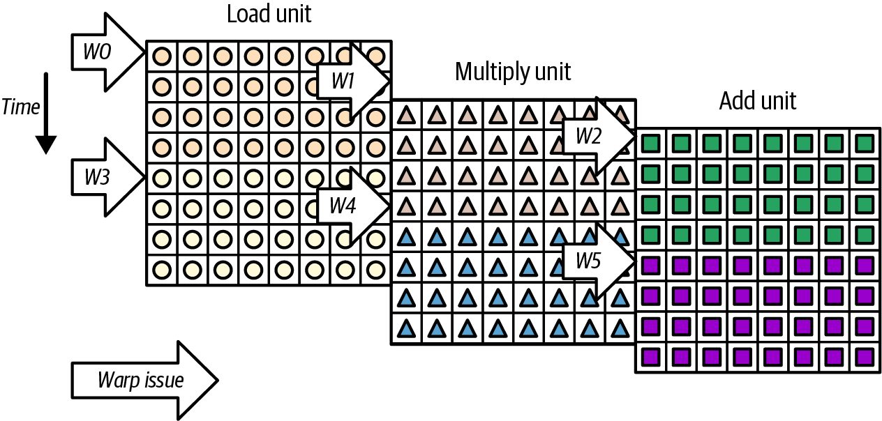
opportunity to execute the second multiply while the first multiply is still in
progress—or while it’s waiting for its operands to load from memory.
This properly overlaps and hides latency. The result is a higher instructions-per-cycle
(IPC) and better latency hiding as shown below by computing the two multiplies,
ai0*bi0 and ai1*bi1, in parallel:
      for (int i = 0; i + 1 < N; i += 2) {
          float ai0 = a[i];        // load a[i]
          float bi0 = b[i];        // load b[i]
          float ai1 = a[i + 1];    // load a[i+1]
          float bi1 = b[i + 1];    // load b[i+1]
          sum += ai0 * bi0 + ai1 * bi1;
      }
Here, we’re loading pairs of values (a[i], b[i] and a[i+1], b[i+1]) before doing any multiplies. Unrolling exposes two independent multiply instructions per loop itera‐ tion. This way, the GPU can overlap those arithmetic operations and hide the latency of each operand load. ILP does not directly change arithmetic intensity (FLOPS per byte). However, it raises overall throughput (FLOPS) by overlapping compute with memory or compute‐to‐ compute dependencies. We explicitly unroll to increase independent work per thread and help dual-issue. In other words, ILP boosts throughput by time-multiplexing independent work—not by doing extra work.
                     A common misconception is that increasing ILP will perform more
                     operations. However, it doesn’t—it just keeps the GPU’s multiple
                     functional units busy. ILP helps only if your program has idle issue
                     slots due to latency. If your kernel is already fully utilizing the exe‐
                     cution units on every cycle (e.g., a tight compute-bound loop with
                     no stalls), increasing ILP won’t actually increase performance.
To encourage the compiler to increase, or expose, ILP, you can use #pragma unroll on short loops or tune ‐maxrregcount to allow the compiler to allocate more registers for holding intermediate values. This explicitly acknowledges that you want the com‐ piler to increase register usage and potentially reduce occupancy. In this way, ILP complements occupancy. High occupancy ensures there are many warps to switch to when one stalls, and ILP makes sure that a single warp can issue as many independent instructions as possible to fill the pipeline and hide latency. This is much like superscalar and out‐of‐order execution in CPUs, except it’s directed explic‐ itly by the compiler’s scheduling of your CUDA code.
326 | Chapter 8: Occupancy Tuning, Warp Efficiency, and Instruction-Level Parallelism
Warp Scheduling and Dual Issue Instructions Each SM contains multiple warp schedulers. For example, Blackwell SMs have four warp schedulers. Each scheduler can issue up to two independent instructions per cycle, as shown in Figure 8-9.
Figure 8-9. Each warp scheduler can dispatch up to two instructions per cycle called “dual issue”
In practice, this means that a single warp can overlap multiple independent opera‐ tions across successive cycles—and sometimes even in the same cycle if they target different pipelines such as one math, one memory, or one special-function unit (SFU) pipeline. This means that multiple instructions can be in flight and progressing through the pipeline simultaneously. This overlap is the ILP that we discussed earlier.
Exposing Instruction-Level Parallelism | 327
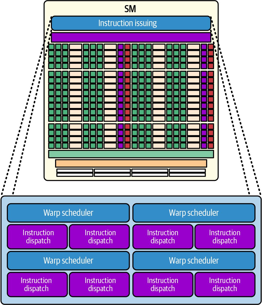
                     On Blackwell, the FP32 and INT32 pipelines have been merged
                     into a single set of unified CUDA cores. As such, they can only exe‐
                     cute either FP32 or INT32 instructions in a given cycle—not both
                     at once. Each core must pick one data type each cycle. As a result,
                     any ILP that depended on dual-issuing an INT and an FP in the
                     same cycle will no longer work since Blackwell must choose one or
                     the other per cycle on each core. As such, mixed INT32 and FP32
                     instruction streams no longer benefit from dual issue on a single
                     core. Mixed streams should instead exploit warp/SM concurrency
                     —and not rely on per-core dual issue. As such, you should prefer
                     dual issue with two independent math and memory instructions
                     (or two independent math instructions such as FP32 and FP16) in
                     flight using ILP. This will increase instruction-issue efficiency.
ILP does not require that two instructions physically fire in the same cycle. Instead, it
makes sure that while one instruction (e.g., long-latency global memory load) is still
pending, the warp can immediately issue another independent instruction (e.g., arith‐
metic operation) on the next cycle.
As a result of this overlap, by the time the data returns from memory, the arithmetic
work has already made progress. This effectively hides the load’s latency. On Black‐
well, multiple instructions can be in flight per warp due to pipelining, and the sched‐
ulers issue to different execution units over successive cycles. In practice, ILP appears
as a steady stream of independent issues rather than a fixed number of concurrent
instructions per warp.
Consider a scenario in which each thread in your kernel loads two array elements—
and then multiplies each by a different constant before combining the results. The
multiply operation for the first element can execute while the second element’s load
operation is still underway.
This overlapping pattern keeps the warps’ execution units busy instead of waiting.
This raises overall throughput without changing how many loads and multiplies
occur per element. Here is a concrete example of increasing ILP:
      // Launch configuration: e.g., 256 threads per block, enough blocks to cover N
      __global__ void independentOps(const float *a, const float *b,
                                     float *out, int N) {
          int i = blockIdx.x * blockDim.x + threadIdx.x;
          if (i < N) {
              float x = a[i];
              float y = b[i];
              // Two independent operations (no dependency between u and v):
              float u = x * x;
              float v = y * y;
              // Dependent operation that uses both results:
              float sum = u + v;
              out[i] = sqrtf(sum);
328 | Chapter 8: Occupancy Tuning, Warp Efficiency, and Instruction-Level Parallelism
} } In this kernel, each thread loads two values x and y from different arrays and com‐ putes two results u and v. The calculations of u = x*x and v = y*y are independent of each other since neither uses the result of the other. Structuring the code this way, instead of sum = x*x + y*y, gives the compiler an opportunity to arrange the instruction sequence to expose ILP and increase perfor‐ mance. Specifically, it can issue the instruction for u = x*x, then in the next cycle issue v = y*y before u has finished. While the first multiplication is running—or waiting for a pipeline slot—the second one can run in parallel in another arithmetic unit. By the time it needs to do sum = u + v, likely both multiplications have been completed. The warp thus had multiple instructions in flight, which helps to hide the latency of those two multiply operations. In contrast, consider the code here in which v’s computation was placed after using u. In this scenario, we’d create an unnecessary dependency chain that limits ILP: float u = x * x; float temp = u + 1.0f; // some dependent use of u float v = y * y;
The kernel computes u = x * x and immediately uses that result to form temp = u + 1.0f. Only after computing temp do you issue v = y * y, which does not depend on u or temp. Therefore, its placement after temp forces the GPU to wait until the u + 1.0f instruction finishes before it can issue the multiply for v. In effect, you create a serial dependency chain: first x * x → u, then u + 1.0f → temp, and only then y * y → v. During the time the hardware is executing (or wait‐ ing for) the u + 1.0f operation, it cannot begin y * y even though v is mathemati‐ cally independent. This ordering artificially limits instruction‐level parallelism because one independent multiply must park itself behind a dependent instruction. By contrast, consider the following reordered and optimized code: // Optimized ordering with better ILP:
    float u = x * x;    // Independent multiply on x
    float v = y * y;    // Independent multiply on y (issues immediately after u)
    float temp = u + 1.0f; // Only now use u
    // ... use v or temp as needed ...
Exposing Instruction-Level Parallelism | 329
Here, we reordered the code such that both x * x and y * y occur back‐to‐back (i.e., float u = x * x; float v = y * y; float temp = u + 1.0f;). In this case, the GPU can issue the two independent multiplies in successive cycles without waiting for the u + 1.0f add to finish. This means that while the result of x * x may still be lingering in a “pending” pipe‐ line slot, the hardware can already start executing y * y. Only once both of those multiplies have calculated their results does the GPU perform temp = u + 1.0f. In other words, you now have two multiplies in flight at once. This fills the execution units and hides latency. This improved ILP, issuing v = y * y as soon as possible, makes sure that the multiply on y overlaps with both the multiply on x and the later add—instead of being forced to wait. Consequently, the warp spends fewer cycles idle, which translates directly into higher throughput. GPUs rely on the compiler, and sometimes the programmer’s hints, to schedule inde‐ pendent instructions. On modern CUDA compilers, simple patterns like the preced‐ ing are usually detected and scheduled optimally. But you can encourage ILP by structuring your code appropriately or using pragma compiler directives. This example is simple, but it demonstrates the idea that you should not serialize independent work within a thread if you can help it. If a thread needs to load two arrays and do math on both, doing them in parallel, or interleaving them, is better than doing one after the other in a serial manner.
ILP and Occupancy On modern GPUs, the maximum resident warps per SM is 64 warps, or 2,048 threads (2,048 threads = 32 threads per warp × 64 warps). The warp schedulers can issue multiple instructions per cycle when dependencies permit. The INT32 and FP32 cores are unified and operate as either FP32 or INT32 in a given clock rather than both at once. The register file per SM is 256 KB, which is 64K 32-bit registers. This large register file is important for sustaining ILP without spilling, as we’ll see in a bit. If you write a kernel with little to no ILP such that each thread issues exactly one operation at a time, you typically need on the order of 1,536 active threads (~48 warps, or 75% occupancy) to saturate the SM’s execution units (these are not hard limits but rather approximations). By contrast, exposing even a modest amount of ILP can significantly lower the num‐ ber of threads required. Table 8-4 summarizes how ILP reduces the threads/occu‐ pancy needed to saturate a Blackwell SM at different ILP values.
330 | Chapter 8: Occupancy Tuning, Warp Efficiency, and Instruction-Level Parallelism
Table 8-4. How ILP reduces the threads/occupancy needed to saturate a Blackwell SM ILP (independent ops/thread) Threads/SM for ~100% utilization Occupancy (% of 2,048 threads) 1 (no ILP) ~1,536 threads (48 warps) 75% 2 ~1,024 threads (32 warps) 50% 3 ~768 threads (24 warps) 37.5% 4 ~512 threads (16 warps) 25%
Here, two-way ILP, in which each thread issues two independent operations back-toback, often achieves full throughput with roughly 1,024 active threads (≈32 warps, or 50% occupancy). This is because each warp keeps two operations in flight whenever one is still pending. Three-way ILP, on the other hand, can saturate with about 768 threads (≈24 warps, or 37.5% occupancy). A four-way ILP may need only 512 threads (≈16 warps, or 25% occupancy) to fill the pipelines. This is because each warp itself does the work of four independent operations.
                   More in-flight operations per thread lets each warp keep the math
                   pipelines busy—even at lower thread counts.
Clearly, increasing ILP lets you achieve peak compute throughput with fewer warps. This is especially valuable when your workload cannot launch huge numbers of threads—or when you want to free up on-chip resources for other tasks. It’s important to note that there is a practical limit on how much ILP you can expose. Even though Blackwell SMs can keep many instructions in flight per warp, each warp can hold only a finite number of pending instructions. On top of that, the compiler must schedule independent instructions without exceed‐ ing the available registers or overwhelming the GPU’s instruction decode bandwidth. The decode bandwidth is the maximum number of instructions per cycle that the instruction‐fetch and decode hardware can push to execution units. Once you hit those limits, adding more independent operations produces diminishing returns. Once you have enough independent work to keep the issue slots and memory system busy, there is little practical benefit in increasing ILP further. Pushing to five-way or six-way ILP produces little gain and can even hurt performance due to the extra reg‐ ister pressure and instruction overhead.
Exposing Instruction-Level Parallelism | 331
                    On Blackwell, the ideal ILP configuration is often between two and
                    four independent operations per thread. At this point, its schedu‐
                    lers and caches are typically saturated. However, the exact point is
                    kernel and workload dependent. Use Nsight Compute issue and
                    stall metrics to decide where to stop.
Loop Unrolling, Interleaving, and Compiler Hinting
To exploit ILP in your own kernels, look for opportunities in which each thread
issues multiple independent arithmetic or memory instructions before any one result
is needed. Common patterns include the following:
Unrolling small loops
   Unrolling loops allows each thread to perform N accumulations (e.g., 2× or 4×)
   with separate accumulator registers. For example, consider the following loop:
          float sum = 0.0f;
          for (int k = 0; k < 4; ++k) {
              float a = A[idx * 4 + k];
              sum += a * w[k]; // dependent on load a
          }
      You can rewrite this to take advantage of ILP, as shown next. This transformation
      creates four independent load-multiply pairs—one per a0..a3—that can be
      issued in rapid succession:
          float a0 = A[idx * 4 + 0];
          float a1 = A[idx * 4 + 1];
          float a2 = A[idx * 4 + 2];
          float a3 = A[idx * 4 + 3];
          float sum0 = a0 * w[0];
          float sum1 = a1 * w[1];
          float sum2 = a2 * w[2];
          float sum3 = a3 * w[3];
          float sum = sum0 + sum1 + sum2 + sum3;
      Here, all four loads are issued first. As each load completes, its corresponding
      multiply can execute and overlap subsequent loads with computations to hide the
      latency of the memory load. In other words, the GPU interleaves these operations
      such that while one pair is waiting on memory, another pair can be multiplying.
      This increases ILP and hides latency.
Interleaving independent operations
     You can interleave operations that use different data elements, as shown here:
          float x = A[idx];
          float y = B[idx];
          // If you wrote float u = x * c; then float v = y * d;,
          // the multiplies are independent.
332 | Chapter 8: Occupancy Tuning, Warp Efficiency, and Instruction-Level Parallelism
        float u = x * c; // can start as soon as x is ready
        float v = y * d; // can start as soon as y is ready, overlapping with u
    Here, you keep the execution units busy on every cycle by not letting one depen‐
    dent instruction block the next independent instruction, etc. In this interleaved
    code, u = x*c and v = y*d are independent instructions and can be executed
    concurrently. The compiler will schedule them back-to-back such that one multi‐
    ply can proceed while the other multiply is still completing. This is ILP in action.
Using compiler hints
    Compiler hints such as #pragma unroll on small loops can help the compiler
    explicitly create multiple arithmetic chains. If needed, you can adjust
    -maxrregcount to allow the compiler to use more registers per thread for the
    unrolled variables. By allowing more resources per thread, you are increasing ILP
    at the cost of fewer threads. This naturally trades off some occupancy for higher
    ILP.
In short, to hide latency and maximize throughput on Blackwell’s deep pipelines, you
should combine high occupancy (e.g., enough warps/threads to hide stalls) with high
ILP (e.g., multiple independent instructions per thread). Here, you make sure that
even when one instruction is waiting (e.g., memory load or long-latency arithmetic),
the warp can issue other instructions immediately. This will significantly increase the
kernel’s achieved FLOPS.
               On large unrolls, watch instruction-fetch and issue stalls in Nsight
               Compute. Excessive unrolling can bloat code size—or saturate
               decode and dispatch—without further throughput gains.
Profiling and Mitigating Register Pressure However, be mindful of register pressure since ILP typically requires more registers to hold multiple independent values and results. If you unroll too much—or add too many parallel computations—you might increase register usage to the point that occupancy falls significantly. As always, finding the right balance is key. The CUDA compiler does a good job of unrolling loops automatically. But if you push ILP too far by manually unrolling too many iterations using #pragma unroll, for instance, you may notice that occupancy drops. In this case, Nsight Compute will show “Limited by Registers” within its Occupancy analysis. This is usually a clear signal that you’ve gone too far. If you see this, you should dial back the unrolling, reduce the number of independent accumulator vari‐ ables, or relax your launch bounds.
Exposing Instruction-Level Parallelism | 333
Specifically, you can reduce the required MinBlocksPerSM or increase MaxThreadsPer Block so that each block can use more registers without spilling. In other words, allow a bit lower occupancy to avoid severe spilling. This way the register pressure eases and occupancy is recovered. From a profiling perspective, if ILP is helping, you should see the “Stall: Exec Dependency” percentage drop since warps are spending less time waiting on prior instructions. And you should see higher instructions per cycle. Nsight Compute reports an Issue Efficiency or IPC metric. This should rise as ILP increases. For example, you should see the issue efficiency or instructions-per-cycle metric rise as you increase ILP. For example, if you see the IPC metric increase from 1.0 to 1.8 per warp scheduler when you unroll, this indicates that the warp is now issuing close to two instructions per cycle on average instead of just one. However, the actual values depend on the instruction mix and the architecture scheduling constraints. You might also see that you can achieve good performance at lower occupancy than before. The ideal scenario is that you have enough ILP to keep each warp busy—and enough warps to keep the SM busy. Between those two, you’re covering latency both within and across warps. At this point, we’ve tackled warp-level parallelism and instruction-level parallelism. These are two ways to keep the GPU’s computational units busy. Next, we turn to measuring and improving arithmetic intensity. This is about maximizing the useful work done per memory access.
Key Takeaways
In this chapter, you saw how to uncover and eliminate GPU kernel bottlenecks by
moving work from slow global memory into faster on-chip resources and compute
units. By following a cycle of profiling, diagnosing, optimizing, and reprofiling, you
can transform kernels from underutilized or memory‐bound into compute‐saturated,
high‐throughput routines. These techniques will help utilize the full power of your
GPUs:
Profiling with Nsight and torch.profiler
    Start with Nsight Systems to visualize end‐to‐end timelines and reveal CPU‐GPU
    gaps, kernel overlaps, and NVTX spans. Then drill into individual kernels with
    Nsight Compute’s stall metrics, roofline analysis, and occupancy reports. In
    PyTorch code, you can insert profiler instrumentation (using the torch.pro
    filer API, built on the Kineto library) to map Python-level operations directly
    to GPU activities. Remember that the PyTorch profiler’s with_flops estimates
    are formula-based on a limited set of operators. It does not read GPU hardware
    counters. For hardware counters, use Nsight Compute on the kernels of interest.
334 | Chapter 8: Occupancy Tuning, Warp Efficiency, and Instruction-Level Parallelism
Tuning occupancy to hide latency
    Adequate warps per SM are essential to cover memory and instruction latencies.
    You can reduce per‐thread register/shared‐memory usage through code refactor‐
    ing or compiler hints. You should also choose block sizes (e.g., 128–256 threads)
    that fit the SM resources. Doing these will increase your kernel’s achieved occu‐
    pancy to an optimal range—around 50%–75%—and stop underutilization (e.g.,
    ~32-48 warps on Blackwell).
Minimizing warp divergence for SIMT efficiency
   Because warps execute in lockstep, any branch divergence means masked lanes
   sit idle. Restructure kernels so that all threads in a warp follow the same path. Use
   predicated operations like ternary math and torch.maximum—or employ warp‐
   vote intrinsics to compact active lanes. This will boost warp execution efficiency
   and reduce serialized execution.
Recognizing performance regimes
    Every kernel falls into one of four buckets: underutilized, latency bound, memory
    bound, or compute bound. This is based on FLOPS, bandwidth usage, and stall
    reasons. Understanding which regime applies will help direct the exact optimiza‐
    tion strategy. For instance, a high Long Scoreboard stall means the workload is
    latency bound.
Exposing ILP
   By unrolling loops, breaking dependency chains, and prefetching data, you
   expose instruction-level parallelism so that each thread can issue multiple inde‐
   pendent operations per cycle. This lets two- or four-way ILP reduce the warps
   needed to fill an SM in half—reducing execution-dependency stalls, raising IPC,
   and decreasing the “Stall: Exec Dependency” metric. Always profile different ILP
   depths alongside thread counts to find your kernel’s sweet spot.
Iterative optimization and validation
     After each change, including occupancy tweaks, ILP restructuring, tiling, or pre‐
     cision scaling, you should reprofile to confirm reduced memory stalls, fewer exe‐
     cution dependencies, and higher achieved occupancy or FLOPS. Always compare
     results to a FP32 baseline using asserts or numeric checks to guard against unac‐
     ceptable accuracy regressions when lowering precision.
Conclusion You saw how effectively tuning GPU performance requires an iterative workflow. First, measure with profilers. Then identify your primary bottlenecks (compute, memory, interconnects, etc.). Last, apply the right optimizations and repeat.
Conclusion | 335
While each new GPU architecture brings improvements in compute and memory bandwidth, they also add complexity. You must constantly stay on top of these inno‐ vations in order to sustain peak performance. We covered how to tune occupancy, avoid warp divergence, and increase ILP. You also saw how to use profilers to correlate CPU, kernel, and NVLink traffic across GPUs. Then we went into Nsight Compute for per-kernel details. In the next chapters, we’ll extend this foundation by focusing on kernel-level effi‐ ciency to increase arithmetic intensity. To do this you will fully utilize the GPUs hardware-optimized resources such as Tensor Cores for compute, TMEM to service the Tensor Cores, and TMA for data transfers. TMA remains the preferred method for bulk copies from global to shared on modern GPUs that support it. Let’s continue pushing toward the hardware’s peak performance limits!
336 | Chapter 8: Occupancy Tuning, Warp Efficiency, and Instruction-Level Parallelism