Ch 10 — Intra-Kernel Pipelining, Warp Specialization, and Cooperative Thread Block Clusters
                                                                      CHAPTER 10
                            Intra-Kernel Pipelining,
                          Warp Specialization, and
                   Cooperative Thread Block Clusters
In the previous chapters, we covered fundamental optimizations such as tuning memory access, maximizing parallelism, overlapping computation and data transfer, boosting occupancy, and minimizing warp stalls. These helped hide latency and elim‐ inate bottlenecks. Modern GPUs, however, offer advanced hardware features and exe‐ cution models that let us take the fundamental optimization techniques even further. In this chapter, we introduce some more advanced CUDA techniques such as warpspecialized pipelines, cooperative groups with grid-level and cluster-level synchroni‐ zation, persistent kernels that loop over dynamic work queues, and thread block clusters (aka cooperative thread array cluster [CTA]) that use distributed shared mem‐ ory (DSMEM or DSM) and Tensor Memory Accelerator (TMA) multicast. At a high level, a thread block cluster is a group of thread blocks that are guaranteed to run concurrently. They can read, write, and perform atomics to each other’s shared mem‐ ory using DSMEM. These methods let us overlap memory accesses and compute operations without host intervention. We can also share data on-chip across thread blocks—and keep every SM fully utilized. By understanding these modern GPU execution models, you’ll be ready to progress to the next chapter where we extend these optimizations even further by exploring inter-kernel pipelines with CUDA streams. The next chapter builds inter-kernel pipe‐ lines on the foundation of intra-kernel optimizations discussed throughout this chapter.
Intra-Kernel Pipelining Techniques Intra-kernel pipelining refers to a set of techniques that overlap memory operations and computations within a single kernel execution. (In the next chapter, we’ll explore inter-kernel pipelining, which overlaps work across multiple kernels running in dif‐ ferent streams.) The core idea is to structure a kernel into concurrent stages such that while one piece of data is being loaded or stored, previously loaded data is being processed. These stages operate in parallel over different tiles or data chunks. This improves through‐ put and efficiently hides latency. Traditionally, GPUs rely on warp-level multithreading to hide latency. While one warp stalls on a memory load, other warps proceed with computation. This is the foundation of single instruction, multiple threads (SIMT) latency hiding in the execu‐ tion model. Intra-kernel pipelining pushes this further by overlapping memory and compute within the same warp or kernel. It uses fine-grained coordination to stagger memory loads and compute—sometimes within a single warp. Intra-kernel pipelining with the CUDA Pipeline API overlaps asynchronous memory transfers and computation without any __syncthreads(). The two common approaches to intra-kernel pipelining are double buffering and warp specialization. In the double-buffered (two stages) pipeline approach, all threads cooperate uni‐ formly. In the warp-specialized pipeline approach, warps are specialized into distinct roles like memory loader, compute, and memory storer. The choice depends on your workload and performance requirements. Table 10-1 summarizes these two <cuda/ pipeline> variants.
Table 10-1. Two approaches for intra-kernel pipelining on modern GPUs using the CUDA Pipeline API API variant Best for Main use Double-buffered pipeline Loop-based tiling and double Overlapping loads and compute in the same warp buffering or block Warp-specialized pipeline (e.g., Persistent kernels with multiple Assigning warps to separate roles/stages such as three-stage memory loader, distinct warp roles (3 in our case) memory load, compute, and memory store compute, memory storer)
374 | Chapter 10: Intra-Kernel Pipelining, Warp Specialization, and Cooperative Thread Block Clusters
Cooperative Tiling and Double-Buffering with the CUDA Pipeline API You can implement the traditional double‐buffered tiling pattern using the C++ Pipe‐ line API by instantiating a two‐stage pipeline to overlap memory loads and computa‐ tions. Specifically, you can declare a two-stage cuda::pipeline_shared_state <cuda::thread_scope_block, 2> object, which is scoped to a specific thread block using cooperative groups (discussed in a bit). This is essentially a producer-consumer pattern, as shown in Figure 10-1.
Figure 10-1. Two-stage producer-consumer pattern with the CUDA Pipeline API
The key CUDA Pipeline API calls are shown next. They are followed by an imple‐ mentation of a double-buffered, cooperative tiling kernel using this API to demon‐ strate modern CUDA techniques that align with hardware features: pipe.producer_acquire() Reserves the next pipeline stage for writing pipe.producer_commit() Signals that the previously issued asynchronous operations for this stage are ready for consumption pipe.consumer_wait() Waits until the previously committed operations for this stage complete to avoid race conditions in loops pipe.consumer_release() Releases the current stage so it can be reused The two stages in the pipeline overlap global-memory loads with computations. In the first, Stage 0, one warp in the thread block issues an asynchronous prefetch for the next tile into shared memory. The prefetch issues cooperative cuda::mem cpy_async copies that lower to per thread cp.async into shared memory.
Intra-Kernel Pipelining Techniques | 375
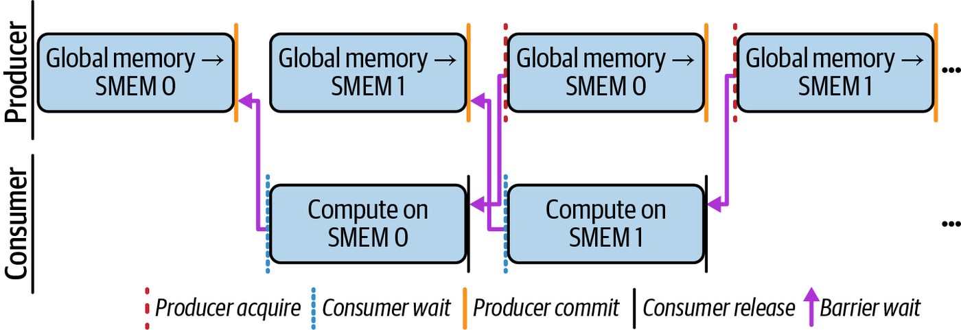
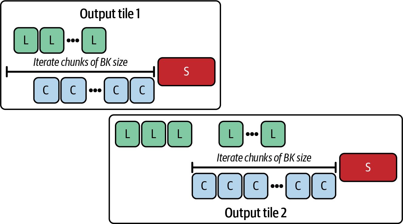
While Stage 0 is producing (loading) the data in one warp, the remaining warps in the thread block are consuming (computing) the loaded data in the second stage, 1. This simple producer-consumer implementation hides DRAM latency with ongoing computations, as shown in Figure 10-2.
Figure 10-2. Hiding global DRAM load (L) latency with (C) compute using a producer– consumer pipeline
This pattern can raise SM utilization and reduce kernel time, but whether you are compute bound or memory bound depends on the operation, tile sizes, and overlap efficiency. Even highly optimized attention kernels like FlashAttention-3 report around 75% percent of peak FP16 FLOPs due to practical limits in overlap and data movement. This is a two-stage, double-buffering example using the CUDA C++ Pipeline API. This API enables the fine-grained producer-consumer synchronization code used here: #include <cuda/pipeline> #include <cooperative_groups.h> #include <algorithm> namespace cg = cooperative_groups;
      #ifndef TILE_SIZE
      #define TILE_SIZE 32
      #endif
      #ifndef STAGES
      #define STAGES 2                    // 2 = double buffer, 3 = triple buffer, etc.
      #endif
      __device__      float computeTile(const float* __restrict__ A_sub,
                                        const float* __restrict__ B_sub,
                                        int tx, int ty) {
376 | Chapter 10: Intra-Kernel Pipelining, Warp Specialization, and Cooperative Thread Block Clusters
    float s = 0.0f;
    #pragma unroll
    for (int k = 0; k < TILE_SIZE; ++k) {
        s += A_sub[ty * TILE_SIZE + k] * B_sub[k * TILE_SIZE + tx];
    }
    return s;
}
extern "C" __global__
void gemm_tiled_pipeline(const float* __restrict__ A_global, // [M x K]
                         const float* __restrict__ B_global, // [K x N]
                         float* __restrict__ C_global,       // [M x N]
                         int M, int N, int K) {
    cg::thread_block cta = cg::this_thread_block();
    // Shared memory layout: A[STAGES] then B[STAGES]
    extern __shared__ float shared_mem[];
    float* A_buf[STAGES];
    float* B_buf[STAGES];
    {
         float* p = shared_mem;
         for (int s = 0; s < STAGES; ++s) {
             A_buf[s] = p;
             p += TILE_SIZE * TILE_SIZE;
       }
         for (int s = 0; s < STAGES; ++s) {
             B_buf[s] = p;
             p += TILE_SIZE * TILE_SIZE;
        }
    }
    __shared__ cuda::pipeline_shared_state<cuda::thread_scope_block, STAGES> state;
    auto pipe = cuda::make_pipeline(cta, &state);
    int tx = threadIdx.x, ty = threadIdx.y;
    int block_row = blockIdx.y * TILE_SIZE;
    int block_col = blockIdx.x * TILE_SIZE;
    float accum = 0.0f;
    int numTiles = (K + TILE_SIZE - 1) / TILE_SIZE;
    // Prologue: load first STAGES tiles (or fewer if short)
    for (int s = 0; s < std::min(STAGES, numTiles); ++s) {
        int aRow = block_row + ty;
        int aCol = s * TILE_SIZE + tx;
        int bRow = s * TILE_SIZE + ty;
        int bCol = block_col + tx;
            pipe.producer_acquire();
            if (aRow < M && aCol < K) {
                cuda::memcpy_async(cta, A_buf[s] + ty*TILE_SIZE + tx,
                                   &A_global[aRow*K + aCol],
                                   cuda::aligned_size_t<32>(sizeof(float)), pipe);
            } else {
                A_buf[s][ty*TILE_SIZE + tx] = 0.0f;
            }
Intra-Kernel Pipelining Techniques | 377
                if (bRow < K && bCol < N) {
                    cuda::memcpy_async(cta, B_buf[s] + ty*TILE_SIZE + tx,
                                        &B_global[bRow*N + bCol],
                                        cuda::aligned_size_t<32>(sizeof(float)), pipe);
                } else {
                    B_buf[s][ty*TILE_SIZE + tx] = 0.0f;
                }
                pipe.producer_commit();
           }
           // Steady state
           for (int tile = 0; tile < numTiles; ++tile) {
               int s = tile % STAGES;
                // Block-scope wait
                pipe.consumer_wait();
                accum += computeTile(A_buf[s], B_buf[s], tx, ty);
                pipe.consumer_release();
                // Prefetch next tile into the same slot s (ring buffer)
                int nextTile = tile + STAGES;
                if (nextTile < numTiles) {
                    int aRow = block_row + ty;
                    int aCol = nextTile * TILE_SIZE + tx;
                    int bRow = nextTile * TILE_SIZE + ty;
                    int bCol = block_col + tx;
                      pipe.producer_acquire();
                      if (aRow < M && aCol < K) {
                          cuda::memcpy_async(cta, A_buf[s] + ty*TILE_SIZE + tx,
                                             &A_global[aRow*K + aCol],
                                             cuda::aligned_size_t<32>{sizeof(float)}, pipe);
                      } else {
                          A_buf[s][ty*TILE_SIZE + tx] = 0.0f;
                      }
                      if (bRow < K && bCol < N) {
                          cuda::memcpy_async(cta, B_buf[s] + ty*TILE_SIZE + tx,
                                              &B_global[bRow*N + bCol],
                                              cuda::aligned_size_t<32>{sizeof(float)}, pipe);
                      } else {
                          B_buf[s][ty*TILE_SIZE + tx] = 0.0f;
                      }
                      pipe.producer_commit();
                }
           }
           // Epilogue: final store (guard tails)
           int cRow = block_row + ty;
           int cCol = block_col + tx;
           if (cRow < M && cCol < N) {
               C_global[cRow * N + cCol] = accum;
           }
      }
378 | Chapter 10: Intra-Kernel Pipelining, Warp Specialization, and Cooperative Thread Block Clusters
The code first retrieves a handle to the current thread block using cooperative groups (CG), discussed in a bit. It then immediately instantiates a two-stage cuda::pipeline object bound to that block. By creating the pipeline before any asynchronous opera‐ tions, the pipelines’ internal barriers and internal synchronization mechanisms are in place prior to performing data movement. The kernel then allocates one contiguous shared-memory region for both A and B tiles by defining an extern __shared__ float shared_mem[]. It divides this buffer into four subregions, two for A and two for B, using pointer arithmetic (float* A_buf[2] and float* B_buf[2]). This allows true double-buffering without extra dynamic allocations. Before entering the main loop, the kernel asynchronously prefetches the first STAGES tiles using asynchronous copies bound to the following pipeline: pro ducer_acquire() → memcpy_async() → producer_commit(). Consumer warps use consumer_wait() and consumer_release() so the compute starts exactly when the prefetched tile is ready. This initial barrier replaces a future need for __syncthreads() and ensures the pipe‐ line’s stage 0 and stage 1 buffers are correctly populated for the first iteration of the producer-consumer sequence. Within each iteration, the kernel reserves the next buffer to load subsequent tiles by calling pipe.producer_acquire(). It then launches two cuda::memcpy_async opera‐ tions—one for the A tile and one for the B tile. Each load is bound to the pipeline object with cuda::memcpy_async(..., pipe), which issues asynchronous copies from global memory into shared memory. These asynchronous copies can overlap well with compute when accesses are coa‐ lesced and tiled correctly. This way, the pipeline stays fed with data to perform maxi‐ mum useful work. Immediately after queuing the memcpy_async calls, the kernel signals completion with pipe.producer_commit(). This commit records the copy’s arrival and allows consumer warps to wait on that specific stage without blocking the entire thread block. Concurrently, other warps in the block invoke pipe.consumer_wait(). This effi‐ ciently stalls only those threads dependent on the data in the curr buffer until the producer has committed it. Once the wait completes, each thread calls the device function computeTile(...) to perform its TILE_SIZE x TILE_SIZE dot-product computation. The results are incrementally accumulated in registers. After finishing the computation on the current buffer, the warps invoke pipe.con sumer_release() to free that stage for reuse in subsequent iterations. This finegrained release prevents block-wide stalls and maximizes overlap between compute and memory transfer phases.
Intra-Kernel Pipelining Techniques | 379
At the end of each iteration, swap the curr and next, which cycles the two doublebuffer stages. This way, the memory buffer that was just computed now becomes the target for the next asynchronous memory. These producer and consumer stages are repeated for all K-dimension tiles. After processing the final tile, each thread’s accumulator contains the full TILE_SIZE x TILE_SIZE dot-product result. This result is then written back to the appropriate ele‐ ment of C_global. When using double buffering, it’s recommended to make sure that each asynchro‐ nous copy (memcpy_async) is followed by the appropriate producer_commit() and consumer_wait() calls for synchronization. This guarantees that the compute kernels will use the data only after it’s properly loaded. Modern CUDA compilers will often perform these optimizations automatically for simple loops.
                    It’s recommended to validate that the pipeline is executing as
                    expected using Nsight Compute’s asynchronous copy metrics. In
                    particular, pay attention to warp occupancy and shared-memory
                    bank conflicts. The goal is to increase SM Active percent and
                    reduce stall cycles. Full hiding of DRAM latency depends on occu‐
                    pancy, access patterns, and shared-memory bank behavior.
This simple double-buffered scheme is roughly 2× faster than naive tiling, as described in Table 10-2’s performance comparison between the naive tiling imple‐ mentation and the optimized, double-buffered, pipeline implementation.
Table 10-2. Performance comparison between the naive tiling and double-buffered kernel using the CUDA Pipeline API Metric Naive tiling Two-stage, double-buffered pipeline (double_buffered_pipeline) Kernel execution time 41.3 ms 20.5 ms (~2× faster versus naive) SM Active % 68% 92% (+24% versus naive)
                    Note: The numeric values in all metrics tables are illustrative to
                    explain the concepts. For actual benchmark results on different
                    GPU architectures, see the GitHub repository.
In this experiment, the gemm_tiled_pipeline kernel using the CUDA C++ Pipeline API achieves a 2× speedup over the naive tiling version. By using the fine-grained pipe.producer_commit() and pipe.consumer_wait() primitives, the pipeline remains filled, and SM Active % jumps 24% from 68% to 92%.
380 | Chapter 10: Intra-Kernel Pipelining, Warp Specialization, and Cooperative Thread Block Clusters
Warp Specialization and the Producer-Consumer Model Warp specialization extends double buffering by assigning operations to warps that use different hardware, such as data movement (e.g., TMA) and compute (e.g., Ten‐ sor Cores). This is in contrast to reusing the same warps for both loading data and computing, as shown in Figure 10-3.
Figure 10-3. Nonwarp specialized kernel with each warp performing a mix of both data loading and compute (source: https://oreil.ly/WZDbM)
This type of specialization allows each set of warps to have their own instruction sequences. As such, instructions are issued and executed continuously without being interrupted by other types of operations. Specifically, warp specialization lets you assign one set of “producer” or “memory” warps to prefetch tiles asynchronously using cuda::memcpy_async. Then all other “consumer” or “compute” warps perform the computations, as shown in Figure 10-4. Here, four warps are assigned the producer role, while the remaining eight warps are assigned the consumer role. Like most producer-consumer patterns, you can assign a different number of warps for the producer and consumer. Because each warp has its own scheduler, the GPU can issue a load instruction, a math instruction, and a write instruction—all in the same cycle from different warps using different warp schedulers. So an SM with multiple schedulers can issue a mem‐ ory instruction from Warp 0, a math instruction from Warp 1, and so on, in one cycle.
Intra-Kernel Pipelining Techniques | 381
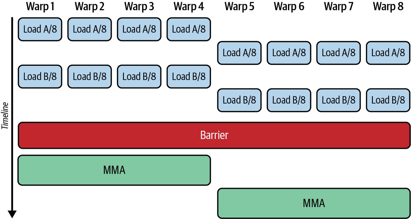
Figure 10-4. Warp-specialized kernel with one set of warps for loading data and all other warps for computations (source: https://oreil.ly/WZDbM)
This effectively creates a thread-block-level multi-issue scenario across warps. This is not possible with single-warp double buffering because a single warp’s scheduler can issue only one instruction per cycle. An interesting pattern for warp specialization is using three different types of warps, such as “loader,” “compute,” and “storer” warps. The loader warp pushes tiles into the pipeline’s queue. The compute warp runs the compute kernel on each tile. And the storer warp writes out the results, as shown in Figure 10-5. This warp-specialized pipeline squeezes out the idle cycles that a single-warp, doublebuffered, sequential load-and-compute loop cannot address. Warp specialization’s efficient overlap of data transfer and computation increases GPU utilization—espe‐ cially for long-running loops and persistent kernels. In these cases, the overhead of role coordination and data handoff is amortized over many iterations. A paper on warp scheduling demonstrated that warp specialization can achieve nearly perfect overlap of memory and compute. In this case, the GPU kernel had dis‐ tinct memory and compute phases such that memory and compute took turns being the bottleneck. By applying warp specialization, their workload transformed into a state in which both the SM’s memory subsystem and compute units were simultane‐ ously busy almost the entire time.
382 | Chapter 10: Intra-Kernel Pipelining, Warp Specialization, and Cooperative Thread Block Clusters
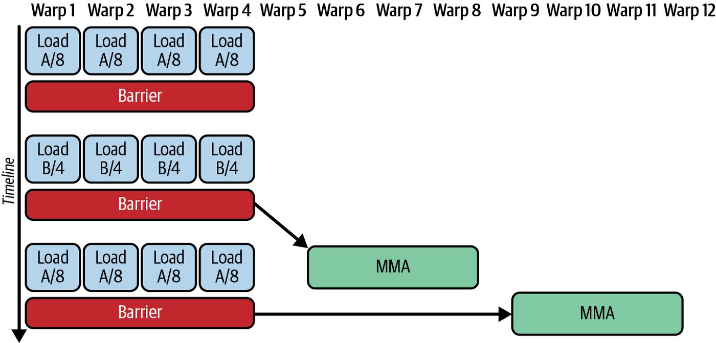
Figure 10-5. Three-role warp-specialized pipeline configuration with one set of warps for loading data, another set for compute, and another set for data storing (source: https:// oreil.ly/xs7YN)
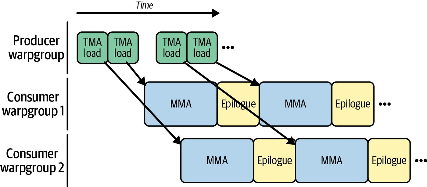
The profiling showed that before using warp specialization, their L2 bandwidth uti‐ lization and Tensor Core utilization were out of phase. After warp specialization, L2 bandwidth and Tensor Core utilization became in-phase. This resulted in much higher effective throughput and showed that warp specialization can squeeze out the last bits of idle time—even for a well-tuned asynchronous pipeline that might be left on the table. Another warp specialization pattern is a modification of the three-role warpspecialized pipeline. It assigns a set of warps to the memory loader as before, but then uses two sets of consumer warps that “ping-pong” between the roles of compute and memory-storer. This three-role warp-specialization architecture is exposed in CUT‐ LASS as gemm_tma_warpspecialized_pingpong and shown in Figure 10-6.
Intra-Kernel Pipelining Techniques | 383
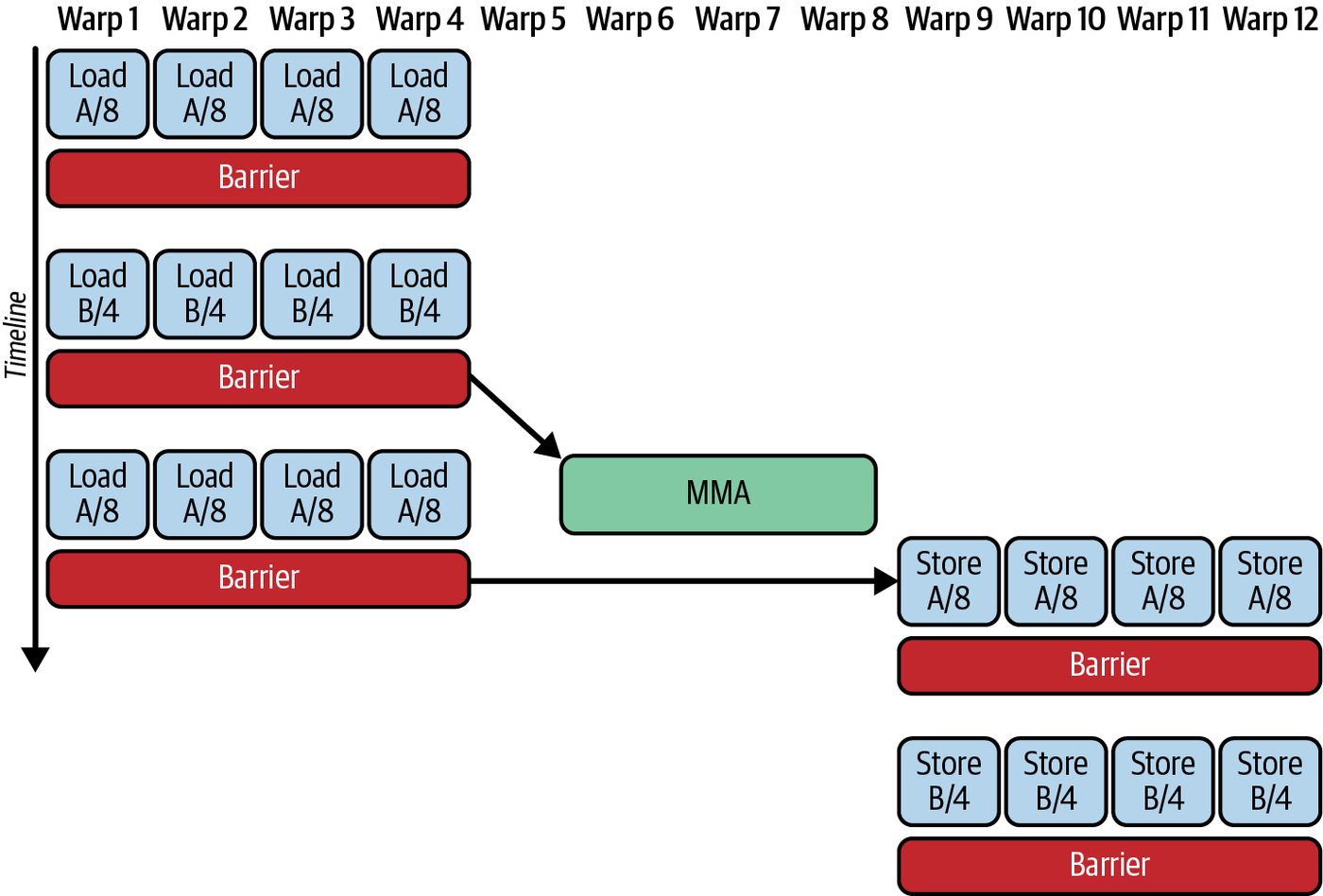
Figure 10-6. Ping-pong architecture with three-role warp-specialized kernel (source: https://oreil.ly/xs7YN)
Here, the consumer MMAs are overlapping and include a small amount of postMMA wrap-up, or epilogue, processing. This per-MMA epilogue cleanup is required before launching the next MMA. Specifically, the epilogue can include accumulating, scaling, writing back to global memory, or shuffling results to another warp. Addi‐ tionally, the epilogue can perform housekeeping like advancing tile pointers, updat‐ ing loop counters, and signaling that this tile is done so the next TMA load or MMA can kick off.
                    While not shown here, there is also an equivalent prologue pro‐
                    cessing step that happens before the MMA operation. In this case,
                    the prologue phase would fill the pipeline with a few TMA requests
                    to move data into registers before the MMA consumers can start
                    doing useful work on the Tensor Cores.
In practice, warp specialization is extremely effective at squeezing out the last bits of performance. In fact, FlashAttention v3 attributes its speedups partially to warpspecialized pipelines that overlap GEMM and softmax computations—along with data transfers—to keep all hardware units busy. This helps achieve near-peak FLOPS for attention computations due to aggressive overlap of compute and TMA-driven data movement. In addition, the PyTorch compiler (covered in Chapters 13 and 14) generates kernels that use warp specialization to schedule separate warps for loading and computing data. It also uses low-cost barriers to synchronize the warps, similar to the CUDA Pipeline API implementation detailed in the next section. The PyTorch compiler sys‐ tem also integrates with CUTLASS’s ping-pong GEMM. Both torch.compile and Triton may generate warp specialized kernels for supported operations. However,
384 | Chapter 10: Intra-Kernel Pipelining, Warp Specialization, and Cooperative Thread Block Clusters
they apply warp specialization selectively based on heuristics and do not enable warp specialization for every operator.
                Use warp specialization for imbalanced or latency-hiding
                scenarios—especially when a single warp’s compute is not enough to
                hide memory-load latency. However, if a kernel is small—or
                extremely memory bound—sticking to a simpler double-buffering
                scheme may produce similar benefits without the extra code
                complexity.
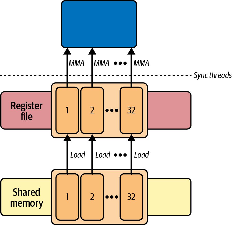
Using CUDA Pipeline API for Warp Specialization Warp specialization builds on the CUDA Pipeline API by allowing specialized warps to communicate using fine-grained producer and consumer primitives. These calls avoid full block barriers while composing naturally with asynchronous copies such as cuda::memcpy_async. The key advantage of using the CUDA Pipeline API’s producer and consumer calls (e.g., pipe.producer_acquire(), pipe.producer_commit(), pipe.consumer_wait(), and pipe.consumer_release()) is that they synchronize only the specific warps or stages that actually need to hand off data. This is in contrast to forcing every thread in a block to wait. A block-wide barrier would stall every warp—even those that are not involved with the producer-consumer pipeline. All execution in that block must pause until every thread reaches the barrier, as shown in Figure 10-7. By comparison, the Pipeline API maintains per-stage state internally. When a pro‐ ducer warp finishes its asynchronous copy and calls pipe.producer_commit, only the warps that call pipe.consumer_wait will block until the data is ready. Other warps in the block can continue running any work that does not depend on that stage. In prac‐ tice, the CUDA Pipeline API reduces idle time and decreases stalled warps because it eliminates the need to pause the entire block with a barrier. With pipelines you coor‐ dinate producer and consumer handoffs at a finer granularity than a hand-coded async-copy sequence (e.g., PTX cp.async + __syncthreads()). You can implement warp specialization with the CUDA Pipeline API in a three-role pattern. A loader warp produces inputs for a compute warp, the compute warp con‐ sumes those inputs and produces results, and a storer warp consumes those results and writes them out. The pipeline object is block scoped, and it tracks the stage order internally.
Intra-Kernel Pipelining Techniques | 385
Figure 10-7. Block-wide barrier prevents threads from proceeding until they synchronize and load the new data
Here is an example of a warp-specialized, three-role kernel that computes tiles of data using a loader warp (warp_id 0), compute warp (warp_id 1), and storer warp (warp_id 2): // warp specialized roles using the CUDA Pipeline API
      #include <cuda/pipeline>
      #include <cooperative_groups.h>
      namespace cg = cooperative_groups;
      // smem_bytes = 3×TILE_SIZE^2×sizeof(float) (three roles, single-pipeline)
      // 3 tiles * 112 * 112 * 4 byte per float =
      // 150,528 bytes < 227,328 bytes (~227 KB)
      // per-block dynamic SMEM limit on Blackwell
      // Choose TILE_* so total shared memory per block is ≤ the device’s
      // reported per-block shared memory limit.
      // Query cudaDevAttrMaxSharedMemoryPerBlockOption and set
      // cudaFuncAttributeMaxDynamicSharedMemorySize accordingly.
      #define TILE_SIZE 112
      // Example tile compute: C = A x B for one TILE_SIZE by TILE_SIZE tile
      __device__ void compute_full_tile(const float* __restrict__ A_tile,
                                        const float* __restrict__ B_tile,
                                        float* __restrict__ C_tile,
                                        int lane_id) {
          for (int idx = lane_id; idx < TILE_SIZE * TILE_SIZE; idx += warpSize) {
386 | Chapter 10: Intra-Kernel Pipelining, Warp Specialization, and Cooperative Thread Block Clusters
        int row = idx / TILE_SIZE;
        int col = idx % TILE_SIZE;
        float acc = 0.0f;
        #pragma unroll
        for (int k = 0; k < TILE_SIZE; ++k) {
            acc += A_tile[row * TILE_SIZE + k] * B_tile[k * TILE_SIZE + col];
        }
        C_tile[idx] = acc;
    }
}
extern "C"
__global__ void warp_specialized_pipeline_kernel(
        const float* __restrict__ A_global,
        const float* __restrict__ B_global,
        float* __restrict__ C_global,
        int numTiles) {
    thread_block cta = this_thread_block();
    // three square tiles in dynamic shared memory: A, B, and C
    extern __shared__ float shared_mem[];
    float* A_tile = shared_mem;
    float* B_tile = A_tile + TILE_SIZE * TILE_SIZE;
    float* C_tile = B_tile + TILE_SIZE * TILE_SIZE;
    // three stage pipeline shared by the block
    __shared__ cuda::pipeline_shared_state<cuda::thread_scope_block, 3>
        pipe_state;
    auto pipe = cuda::make_pipeline(cta, &pipe_state);
    int warp_id = threadIdx.x >> 5;
    int lane_id = threadIdx.x & 31;
    int warps_per_block = blockDim.x >> 5;
    // grid wide warp indexing for persistent tiling
    int totalWarps = gridDim.x * warps_per_block;
    int global_warp = warp_id + blockIdx.x * warps_per_block;
    for (int tile = global_warp; tile < numTiles; tile += totalWarps) {
        size_t offset = static_cast<size_t>(tile) * TILE_SIZE * TILE_SIZE;
        if (warp_id == 0) {
            // loader produces A_tile and B_tile
            pipe.producer_acquire();
            auto bytes = TILE_SIZE * TILE_SIZE * sizeof(float);
            cuda::memcpy_async(cta, A_tile, A_global + offset,
                               cuda::aligned_size_t<32>{bytes}, pipe);
            cuda::memcpy_async(cta, B_tile, B_global + offset,
                               cuda::aligned_size_t<32>{bytes}, pipe);
            pipe.producer_commit();
        }
Intra-Kernel Pipelining Techniques | 387
                if (warp_id == 1) {
                    // wait for A_tile/B_tile
                    pipe.consumer_wait();
                    // compute C_tile from A_tile, B_tile
                    compute_full_tile(A_tile, B_tile, C_tile, lane_id);
                    // finished consuming A/B; free that stage
                    pipe.consumer_release();
                    // publish C_tile for the storer warp
                    pipe.producer_acquire();
                    pipe.producer_commit();
                }
                if (warp_id == 2) {
                    // store consumes computed C_tile
                    // Wait for the committed stage before consuming
                    pipe.consumer_wait();
                    for (int idx=lane_id; idx<TILE_SIZE*TILE_SIZE; idx+=warpSize) {
                        C_global[offset + idx] = C_tile[idx];
                    }
                    pipe.consumer_release();
                }
           }
           // launch with dynamic shared memory size equal to
           // 3 * TILE_SIZE * TILE_SIZE * sizeof(float)
           // When launching with dynamic shared memory >48 KB
           // You need to set cudaFuncAttributeMaxDynamicSharedMemorySize
           // for the kernel
      }
Here each warp works in a distinct role. The loader warp calls producer_acquire(), performs two cooperative copies with cuda::memcpy_async into A_tile and B_tile, then calls producer_commit(). The compute warp calls pipe.consumer_wait() to observe the newly committed data and immediately calls consumer_release() to free that stage for reuse. The compute warp then becomes a producer for the next handoff by calling producer_acquire(), computing C_tile, and calling producer_commit(). The storer warp calls consumer_wait() to observe the computed C_tile and writes it to global memory in a warp-striped loop, then calls consumer_release(). This sequence uses a single block-scoped pipeline with no explicit stage numbers, and it avoids any blockwide __syncthreads.
                     This kernel runs as a persistent kernel across many tiles to amortize
                     launch overhead. More on persistent kernels in a bit.
388 | Chapter 10: Intra-Kernel Pipelining, Warp Specialization, and Cooperative Thread Block Clusters
In short, using the CUDA Pipeline API together with cooperative groups allows fine‐ grained, SM‐wide producer‐consumer handoffs without any explicit __sync threads() calls. Table 10-3 compares three implementations: a naive tiled kernel, a two‐stage double‐buffered GEMM using double_buffered_pipeline, and our warp‐ specialized pipeline kernel warp_specialized_pipeline.
Table 10-3. Comparison of three implementations: a naive tiled kernel, a two‐stage double‐ buffered GEMM, and a warp‐specialized pipeline kernel Metric Naive Two‐stage, double‐buffered pipeline Warp‐specialized pipeline tiling (double_buffered_pipeline) (warp_specialized_pipeline) Kernel 41.3 ms 20.5 ms (2.01× faster versus naive) 18.4 ms (10.2% speedup versus two‐stage) execution time Warp execution 68% 92% (+24% versus naive) 96% (+4% versus two‐stage) efficiency Shared memory High Low Minimal stall latency/ warp sync stalls L2 throughput 80 GB/s 155 GB/s (+94% versus naive) 165 GB/s (+6.45% versus two‐stage) Throughput Scales up Scales well up to ~6 warps per SM Scales nearly linearly to the SM’s warps (e.g., scalability to only 2– 64 warps) 3 warps per SM DRAM bytes Poor Great overlap Excellent overlap read versus SM overlap cycles Instruction 1.7 B 1.05 B (–38% versus naive) ~1.00 B (–5% versus two‐stage) count
Here, the double‐buffered pipeline finishes GEMM in 20.5 ms, whereas the warp‐ specialized version completes in just 18.4 ms. This 10.2% improvement is a result of the warp-specialized kernel only stalling the consumer warp (e.g., compute). The other warps (e.g., loader and storer) progress independently. In the previous twostage, double-buffered kernel, every thread participates in the consumer phase. As such, consumer_wait() effectively stalls the entire thread block. This finer‐grained, per‐warp synchronization eliminates the implicit full‐block wait and allows all three warps (loader, compute, and storer) to overlap continuously. As a result, average SM utilization rises from roughly 92% in the double‐buffered design to about 96% in the warp‐specialized version—and warp‐stall cycles drop to near-zero. From a scalability standpoint, Nsight Compute shows that the naive tiling kernel sat‐ urates after just two to three active warps per SM. This is because each tile load must complete before any computation can start.
Intra-Kernel Pipelining Techniques | 389
The two‐stage, double‐buffered kernel improves on this by overlapping loads and compute. This implementation scales up to 6 warps per SM before shared‐memory or register limits become an issue. In contrast, the warp_specialized_pipeline scales almost linearly as long as you can assign additional warps for load, compute, and store. On Blackwell, for instance, you can keep up to the architectural limit of 64 resident warps per SM. (Actual residency depends on registers, shared memory, and block size.) As Table 10-3 shows, both the double‐buffered and warp‐specialized approaches sub‐ stantially outperform the naive tiled kernel. The double_buffer_pipeline halves the runtime by overlapping tile loads and computation, while the warp_special ized_pipeline adds another 10.2% speedup by avoiding any implicit block‐wide waits. Only the dedicated “compute” warp ever stalls. Instruction counts drop from 1.7 billion in the naive version to 1.05 billion in the two‐stage pipeline, a 38% reduction, and further to ~1.00 billion in the warp‐ specialized kernel for an additional 4.76% reduction. L2 load throughput climbs from 80 GB/s in naive tiling to 155 GB/s in the two‐stage approach (+94%) and then to 165 GB/s in the warp‐specialized kernel (+6.45% versus two‐stage). This is because this warp-specialized kernel dedicates one warp to loading each tile into shared memory once—and then multicasts that single copy to all com‐ pute lanes. This eliminates any remaining redundant L2 reads. As such, after tiling and double-buffering, nearly all redundancy is already removed from the pipeline. In practice, the two‐stage double‐buffered pipeline is ideal for uniformly tiled GEMM workloads. Its simpler producer/consumer model hides most of the DRAM latency under compute. Meanwhile, the warp‐specialized approach is optimized for irregular or deeper pipelines such as fused attention kernels. This is because each warp can continuously perform its assigned role—loading, computing, or storing—without ever forcing the rest of the block to stall.
PyTorch, CUDA Pipeline API, and Warp Specialization PyTorch’s public API doesn’t expose cuda::pipeline directly, but when you invoke torch.compile, the compiler generates kernels (implemented in OpenAI’s Triton lan‐ guage) that use optimizations that implement functionality equivalent to <cuda/pipe line> primitives and warp‐specialized producers/consumers. So while you won’t see cuda::pipeline calls explicitly generated, you will see the underlying instructions and barriers. These optimizations help to improve occupancy and increase data-transfer/computation overlap. In other words, you get the same low‐latency, high‐throughput behavior of a handwritten <cuda/pipeline> imple‐ mentation without writing any CUDA code yourself.
390 | Chapter 10: Intra-Kernel Pipelining, Warp Specialization, and Cooperative Thread Block Clusters
PyTorch’s fused attention kernels, produced by TorchInductor, use warp specializa‐ tion with producer and consumer groups. For instance, consider three separate GPU kernels in PyTorch shown here: scores = torch.matmul(queries, keys.transpose(-2, -1)) probabilities = F.softmax(scores, dim=-1) context = torch.matmul(probabilities, values) You can simply rewrite this with one line in PyTorch as shown here: context = torch.nn.functional.scaled_dot_product_attention(queries, keys, values) Under the hood, the loader warps fetch tiles into shared memory. the compute warps process the tiles, and the store warps write results back. This eliminates expensive round trips to global memory between matmul and softmax stages. Overall, torch.compile is ideal for performance‐sensitive and irregular workloads. Modern GPUs like Blackwell have abundant SM resources and high memory band‐ width. As such, techniques like warp specialization minimize idle cycles and allow near-linear scaling across warps—at least until the SMs—or memory bandwidth—are fully saturated.
               Even highly optimized kernels like FlashAttention-3 reach only
               about ~75% of peak FP16 FLOPS using warp-specialized overlap.
               This shows that you don’t need to achieve 100% compute utiliza‐
               tion to achieve a significant optimization milestone.
By decoupling load, compute, and store into independent stages, the pipeline model maximizes throughput and resource utilization, making it the preferred approach for long‐running kernels, including such processes as transformer attention, fused opera‐ tor pipelines, and custom task schedulers. These kernels use the fine‐grained inter‐warp communication, deep pipelining, and linear warp scaling to provide high performance.
Persistent Kernels and Megakernels Persistent kernels, also called persistent threads, invert the usual one-kernel-per-task approach. Instead of launching many small kernels in which each incurs significant overhead, you can launch a single, long‐running kernel whose threads continually pull work from a shared producer-consumer queue in global or shared memory. When persistent threads loop, they handle data chunks as they arrive—often using memory copies or host signals—without exiting the kernel. This avoids repeated ker‐ nel launch overhead entirely. For instance, a persistent kernel might use one thread block’s Warp 0 to copy data from global memory (or CPU host memory) to shared
Persistent Kernels and Megakernels | 391
memory. In the meantime, Warp 1 computes the previous batch. This is a form of software pipelining on GPU. For instance, consider having 1,000 tiny, independent tasks. Traditionally, one might launch 1,000 separate kernels. Each kernel occupies only a few SMs for a brief moment before exiting. In practice, the GPU would repeatedly ramp up for each tiny kernel and ramp down afterward. This would leave most SMs idle between launches—and would fail to uti‐ lize the hardware fully. With a persistent kernel, you instead launch one large grid designed to keep the GPU busy for the entire workload. On a GPU with 132 SMs, for instance, this might mean launching one block per SM with 256 threads per block. That’s 33,792 threads in total. Each thread then executes code that looks roughly like the following: __device__ int g_index; // global counter for next task; initialize to 0 on host
      __global__ void persistentKernel(Task* tasks, int totalTasks) {
          // Every thread loops, atomically grabbing next task index until none remain
          while (true) {
              int idx = atomicAdd(&g_index, 1);
              if (idx >= totalTasks) break;
              processTask(tasks[idx]);
          }
      }
Before launching this kernel, the host would set g_index = 0 in device memory. It would then invoke the kernel as shown here: cudaMemset(&g_index, 0, sizeof(int));
      // one block per SM on a 132 SM GPU
      int blocks         = 132;
      int threadsPerBlock = 256;
      persistentKernel<<<blocks, threadsPerBlock>>>(d_tasks,
          totalTasks);
cudaDeviceSynchronize(); Now, instead of paying launch overhead for every single task, you pay only once to launch the persistentKernel. Assuming the launch takes roughly 0.02 ms and each of the 1,000 tasks runs in 0.1 ms, the kernels would run back to back for approxi‐ mately 100 ms of total work.
392 | Chapter 10: Intra-Kernel Pipelining, Warp Specialization, and Cooperative Thread Block Clusters
By comparison, running 1,000 tiny kernels back to back, each taking 0.02 ms to launch, would add 20 ms in overhead to the execution time—separate from the 100 ms of total runtime for all 1,000 tasks. In short, consolidating small tasks into a per‐ sistent loop can cut tens of milliseconds of launch overhead. Using persistent kernels, the GPU stays highly utilized—with nearly all SMs actively working on tasks concurrently—because tens of thousands of threads are available to process the ~1,000 tasks. In contrast, launching 1,000 tiny kernels sequentially leaves much of the GPU underutilized at any given time. In our example this equates to only ~35% of the GPU’s capacity being used on average. In this persistent kernel scenario, each SM is running one block of 256 threads (out of 2,048 total threads max), so every SM is doing work. As such, nearly 100% of SMs are active even though each SM’s own occupancy is relatively low at 12% (256 ÷ 2048 threads.) Using persistent kernels in this manner, the GPU can maintain high measured SM Active percent, subject to register and shared memory usage. Remember to always verify with Nsight Compute. On modern GPUs, persistent kernels are particularly effective because their larger shared‐memory capacity and expanded register file allow each thread to hold more intermediate state on‐chip. Threads can use TMA to prefetch tensor tiles for upcom‐ ing tasks while other warps compute. So while some threads are processing one task, other threads use TMA to prefetch data for upcoming tasks—without burdening the SM’s compute pipelines with memory transfer instructions.
Common Workloads for Persistent Kernels Persistent kernels shine when you have many small or unevenly sized tasks that would incur high launch overhead if handled separately. They allow dynamic load balancing. This allows faster threads to continue looping and grab more work. Using persistent kernels, no SM ever goes idle prematurely. This pattern is common in irregular workloads such as graph traversals, custom batched transformations, and per‐token operations common in LLM inference. In these cases, each task’s time can vary significantly. There are downsides to persistent kernels, however. First, you must explicitly manage your task queue and synchronization using atomics. This can introduce contention if many threads attempt to increment the same counter simultaneously.
Persistent Kernels and Megakernels | 393
Debugging a single, giant persistent loop is more complex than debugging multiple small kernels. This is because a single divergent thread or an unexpected branch can cause the entire kernel to hang. Furthermore, one persistent kernel can monopolize the GPU indefinitely. So if other workloads need to run concurrently, you must care‐ fully assign streams or partition resources. In short, persistent kernels can increase overall throughput substantially (e.g., 2–3×) compared to naive kernels by turning the GPU into a dynamic “worker‐thread” pool that continuously fetches and processes tasks. On modern GPU hardware, this approach eliminates launch overhead, maximizes SM occupancy, and—when com‐ bined with cooperative groups or thread block clusters (described in a bit)—keeps data on‐chip throughout multistage pipelines. More and more frameworks and libraries are using persistent kernels and megaker‐ nels to avoid wasted capacity and improve performance of latency-sensitive work‐ loads like inference. The key is to eliminate repeated launches and use device-side task queues on the GPU to keep the SMs fully occupied and performing useful work.
                     As of this writing, PyTorch does not automatically fuse an entire
                     multistage workload into one kernel due to scheduling complexity.
                     As such, achieving the full benefits of persistent kernels and mega‐
                     kernels requires custom CUDA code or specialized compilers. Nev‐
                     ertheless, for multiphase algorithms, refactoring into persistent
                     megakernels can produce significant performance gains—as long
                     as you properly handle synchronizations and avoid deadlocks.
Megakernels for Inference Additionally, a modern approach to persistent kernels originating from large-scale inference is called a megakernel. A megakernel fuses entire sequences of operations across layers—and even across GPUs—into a single large kernel. As shown in Figure 10-8, persistent megakernels have shown to reduce latency by 1.2× to 6.7× ver‐ sus traditional per-layer launches by eliminating repeated kernel launch overhead.
394 | Chapter 10: Intra-Kernel Pipelining, Warp Specialization, and Cooperative Thread Block Clusters
Figure 10-8. Decode throughput improvement with megakernels relative to vLLM and SGLang (source: https://oreil.ly/2aZiF)
Persistent Kernels and Warp Specialization Warp specialization is typically used with persistent kernels in which threads perform many iterations over a relatively long period of time. This allows for deeper pipelines, better overlap, and efficient utilization of long-lived resources. For shorter-running kernels, the added code complexity of persistent kernels and warp specialization might not pay off. And a limitation of persistent-kernel scheduling is finding enough SMs for the persis‐ tent kernel to utilize. If too many SMs are occupied by another kernel, there might not be enough resources for the persistent kernel to launch. This makes it challenging when trying to schedule and load-balance work across SMs. To facilitate persistent kernels (and therefore warp specialization), modern GPUs support thread block clusters—also called cooperative thread array (CTA) clusters since a thread block is also called a cooperative thread array. We will discuss thread block (CTA) clusters in an upcoming section, but, in short, they let you combine thread blocks into “clusters” that occupy multiple nearby SMs on the GPU.
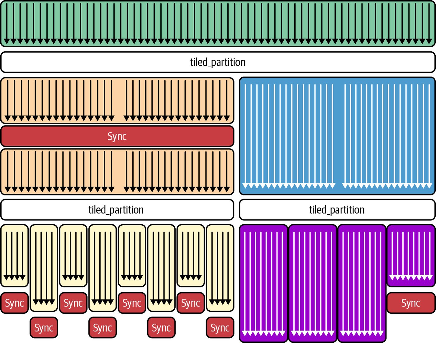
Cooperative Groups Cooperative groups let you define and synchronize groups of threads at arbitrary granularities. For example, you can create groups with individual threads, warps, tiles, blocks, and clusters, as shown in Figure 10-9.
Cooperative Groups | 395
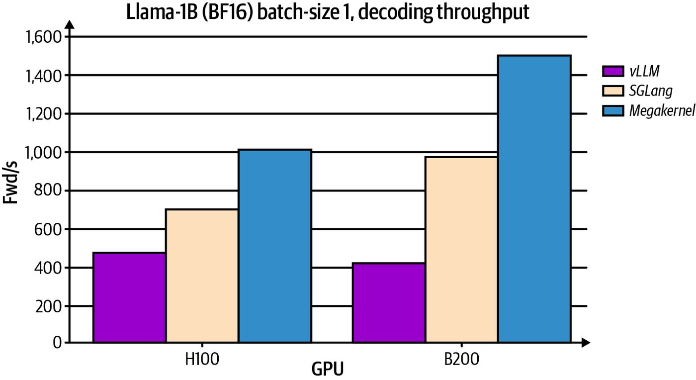
Figure 10-9. Synchronizing across different granularities of threads using cooperative groups
Cooperative groups provide safe, reusable collectives like sync, broadcast, and reduce. This is in contrast to using ad hoc synchronization barriers. Normally, threads can only synchronize within their own block using __syncthreads()—and there is no built-in global barrier for the entire grid, for example. Cooperative groups give you fine-grained synchronization inside the kernel. The API is ideal for coordinating multistage pipelines across warps, blocks, and clusters. To use the Cooperative Groups API with your kernels, you simply include <coopera tive_groups.h>, obtain group objects, then synchronize and coordinate across these groups. The API includes calls like cg::this_thread_block(), cg::tiled_partition(), and cg::this_cluster(). You then call group.sync()—or similar collectives—to coordi‐ nate the threads in these groups. To launch a kernel in cooperative mode, you use cudaLaunchCooperativeKernel(). In cooperative mode, CUDA ensures the grid you launch can be resident concur‐ rently—otherwise, the launch fails. As such, it’s recommended to always size the
396 | Chapter 10: Intra-Kernel Pipelining, Warp Specialization, and Cooperative Thread Block Clusters
cooperative grid using cudaOccupancyMaxActiveBlocksPerMultiprocessor and clamp grid size to avoid launch failure. Inside the kernel, you can then call the follow‐ ing to implement an all-thread-block barrier: cooperative_groups::this_grid().sync(); // or grid.sync() In this case, no thread in any block can proceed past that point until every thread in every block has reached it. This barrier allows you to split a kernel into sequential phases without ending the launch or returning control to the host. For instance, consider the softmax algorithm, common in LLMs, that has two stages: a reduction across the entire array to compute an aggregate sum, and then a subse‐ quent per-element computation that uses the aggregate sum. Traditionally, you would launch one kernel to do the reduction, copy the result back to host memory or global memory, launch a second kernel to consume the result from host or global memory, then calculate the softmax. This requires a lot of relatively slow memory movement. With cooperative groups, you can perform both stages in one kernel such that each block computes its partial sum, one block aggregates those partial sums into a final result, all blocks call grid.sync() to wait until aggregation is complete, then all threads proceed to the second stage. Each thread would then read the aggregate sum from a register or shared memory—rather than from global memory. CUDA guarantees that every block in a cooperative launch is resident on the GPU at the same time. If you request more blocks than can fit concurrently, the launch sim‐ ply fails. Because cooperative kernels must be launched with a grid size that the GPU can run concurrently, grid.sync() will not hang waiting for nonexistent blocks. In other words, the CUDA runtime guarantees that all thread blocks are active and will reach the grid.sync() barrier. If the kernel launch were too large to run at once, it would simply fail to launch. As such, it’s important to check the return status of cudaLaunch CooperativeKernel(). For instance, if a GPU has 132 SMs and your kernel uses enough resources that each SM can run four blocks, the grid must be no larger than 528 blocks to succeed. If you exceed that limit, the cooperative launch will simply fail. Use cudaOccupancyMax ActiveBlocksPerMultiprocessor to size the grid for a cooperative kernel and check the cudaLaunchCooperativeKernel return status before assuming progress has been made. Prior to Blackwell, developers often used cudaLaunchCooperativeKernel together with global-memory atomics or flags to coordinate multiple blocks that did not share on-chip memory. This approach worked but forced intermediate results to be moved to global memory. This incurred extra HBM traffic.
Cooperative Groups | 397
On Blackwell, thread block clusters and DSMEM provide a far more efficient alterna‐ tive. A thread block cluster can share data in on-chip SRAM—and synchronize without global memory round trips. We will cover thread block clusters and DSMEM later in this chapter. You should use cooperative kernels when you need a true, all-thread-block barrier within a single kernel launch. Also, they’re useful when you want to keep intermedi‐ ate results in fast memory (e.g., registers or shared memory) rather than repeatedly writing to and reading from global memory. It’s recommended that you constrain your grid size to the GPU’s maximum concurrent block capacity—or choose larger blocks—to reduce overall block count and a failed kernel launch. The downsides of cooperative kernels are that your grid size is limited by capacity. This may force you to use fewer, larger blocks—or rely on thread block clusters (later in this chapter). Even though all blocks run concurrently, a cooperative barrier still requires every thread in every block to call grid.sync(). If any single thread skips—or never rea‐ ches—the grid.sync() call (e.g., because of a divergent if statement), then every other thread that did call grid.sync() will wait forever. This results in a deadlock. In short, cooperative group kernels let you treat the entire GPU as a single collabora‐ tive resource, with grid.sync() acting as a global barrier. This is ideal for multistage algorithms requiring global synchronization and data sharing. Just remember that grid.sync() is a relatively heavyweight synchronization with higher overhead than block-scoped or cluster-scoped barriers. This is because it must coordinate across all thread blocks running on multiple SMs. As such, you should use grid.sync() spar‐ ingly and, at the very least, make sure that your kernel does a significant amount of work between heavyweight synchronization calls.
                     For cases where you need only limited cross‐block coordination,
                     using global‐memory atomics or per‐block flags can be safer and
                     simpler than relying on a full‐grid barrier. However, they are less
                     efficient than using thread block clusters and DSMEM, as we’ll dis‐
                     cuss in a bit.
Cooperative Grid Synchronization and Persistent Kernels If your workload occasionally needs cross‐thread-block barriers inside a persistent loop to aggregate partial results, you can combine persistent kernels with cooperative groups by calling grid.sync(). This will provide a grid-wide barrier to avoid ending the kernel and having to relaunch it. In this way, a multistage pipeline of reductions and other global steps remains entirely on‐device.
398 | Chapter 10: Intra-Kernel Pipelining, Warp Specialization, and Cooperative Thread Block Clusters
For instance, consider a workload that performs two different computations repeat‐ edly across 1,000 iterations such that each computation requires a global barrier because of cross-block data dependencies. A naive implementation might launch two separate kernels per iteration, resulting in 2,000 kernel launches. In a single stream, the second kernel waits for the first automatically—no explicit host-side sync—but you still pay launch overhead. Instead, you can fuse everything into one cooperative, persistent kernel, as shown here: #include <cuda_runtime.h> #include <cooperative_groups.h> namespace cg = cooperative_groups;
    __device__ inline float someComputationA(float x) { return x * 2.0f; }
    __device__ inline float someComputationB(float a, float b) { return a + b; }
    __global__ void combinedKernel(float* __restrict__ dataA,
                                   float* __restrict__ dataB,
                                   int N,
                                   int iterations) {
        cg::grid_group grid = cg::this_grid();                 // whole-grid group
        const int tid = blockIdx.x * blockDim.x + threadIdx.x; // thread's linear id
        const int stride = gridDim.x * blockDim.x;             // total grid threads
        for (int it = 0; it < iterations; ++it) {
            // Stage 1: update all elements of A using a grid-stride loop
            for (int i = tid; i < N; i += stride) {
                dataA[i] = someComputationA(dataA[i]);
            }
grid.sync(); // global barrier; also provides memory visibility
            // Stage 2: use finished A to update B (again grid-stride)
            for (int i = tid; i < N; i += stride) {
                const float mid = dataA[i];
                dataB[i] = someComputationB(mid, dataB[i]);
            }
            grid.sync();   // barrier before next iteration
        }
    }
On the host side, you would simply invoke this combined cooperative and persistent
kernel, as shown here:
    // ... allocate/copy dA, dB, set N, iterations, choose blockSize
    cudaDeviceProp prop{};
    cudaGetDeviceProperties(&prop, 0);
    if (!prop.cooperativeLaunch) {
        // Fallback: run two kernels per iteration instead of grid.sync()
        // (see alternative below)
    }
Cooperative Groups | 399
      // Compute the maximum grid size allowed for a cooperative kernel
      int maxBlocksPerSm = 0;
      const int blockSize = 256;
      cudaOccupancyMaxActiveBlocksPerMultiprocessor(&maxBlocksPerSm,
                                                    combinedKernel,
                                                    blockSize, 0);
      const int maxCoopGrid = maxBlocksPerSm * prop.multiProcessorCount;
      // Choose grid size, but clamp to cooperative limit
      int gridSize = (N + blockSize - 1) / blockSize;
      if (gridSize > maxCoopGrid) gridSize = maxCoopGrid;
// Launch cooperatively void* args[] = { &dA, &dB, &N, &iterations }; cudaLaunchCooperativeKernel((void*)combinedKernel, gridSize, blockSize, args); cudaDeviceSynchronize(); This single kernel replaces what would otherwise be 2 × 1,000 = 2,000 kernel launches and avoids repeated launch overhead. Inside the loop, grid.sync() ensures correct ordering (every block finishes Stage 1 before any block begins Stage 2—and before the next iteration) without any host-side synchronization. Per-thread and per-block data can remain in registers/shared memory across grid.sync(). For cross-block data exchange, use global memory (or thread block clusters and distributed shared memory, as we’ll cover in a bit). Meanwhile, because the work is looped on the GPU, there is no launch overhead after the first invocation. Cooperative kernels require device support (cooperativeLaunch) and must be launched with cudaLaunchCooperativeKernel. All blocks in the grid must be resi‐ dent concurrently. Size and clamp the grid using the CUDA Occupancy APIs so all CTAs can co-reside. Otherwise the launch will fail. An example is when ((N + threads - 1) ÷ threads) exceeds the cooperative capacity.
Use the CUDA Occupancy APIs to size cooperative grids.
Modern GPUs can run on the order of a few thousand thread blocks concurrently (assuming each uses a modest amount of resources, including registers and shared memory), so there is considerable headroom. However, you should still verify block size and resource consumption before proceeding with this implementation. In this kernel example, the kernel never returns control to the host between itera‐ tions. As such, it behaves like a persistent kernel for the outer loop but enforces global synchronization points in the inner stages.
400 | Chapter 10: Intra-Kernel Pipelining, Warp Specialization, and Cooperative Thread Block Clusters
This combined pattern is especially powerful for multistep algorithms in LLM infer‐ ence in which each layer may require a reduction or normalization (Stage 1) followed by a per-element transformation (Stage 2). By capturing everything in a cooperative persistent kernel, you eliminate all inter-kernel round trips and maximize on-chip data locality.
When to Combine Persistent Kernels and Cooperative Groups A common best practice is to launch a persistent kernel with one thread block per SM if resources allow. This way, each SM has a resident thread block that iteratively pro‐ cesses tasks from a work queue. This maximizes occupancy and keeps SMs from becoming idle. The thread blocks would then use grid.sync() to coordinate between their phases. However, when deciding between cooperative and persistent strategies— and whether to combine them—ask the following questions: Do you have multiple sequential phases that need global synchronization? If yes, use cooperative kernels (or cooperative persistent kernels) so you can call grid.sync() between phases. Do you have many small or irregular tasks that suffer from launch overhead? If yes, use persistent kernels so your threads loop over a shared queue without returning to the host. Can you afford to reserve the entire grid (or a thread block cluster) exclusively for this workload? If yes, a cooperative persistent kernel may yield the best performance. Do you need to share SMs with other work? If yes, consider using thread block clusters (next section) so the persistent or cooperative kernel does not serve other workloads. In short, when you use a single kernel that both loops persistently over tasks and includes grid.sync() calls to synchronize all thread blocks between stages, you elim‐ inate the pauses and extra memory transfers that normally occur between separate kernel launches. With modern GPUs, this means data stays in shared memory or registers throughout the entire computation. This is in contrast to writing the data back to global memory after each phase. As a result, the GPU stays busy doing useful work almost all the time—achieving performance close to its peak hardware limits. One important caveat: cooperative kernels reserve all SMs in the grid, so no other kernels can run concurrently on those SMs. If you need to coschedule other work such as asynchronous data prefetch on a separate stream or lower-priority inference kernels, you may need to partition the GPU into thread block clusters, covered in the next section.
Cooperative Groups | 401
Thread Block Clusters and Distributed Shared Memory A cooperative group is a software-level abstraction that provides an API that lets you carve up kernel threads into arbitrary collectives for synchronization and data move‐ ment. This includes warps, tiles, thread blocks—even entire grids or multidevice grids. In contrast, a thread block cluster (or cooperative thread array [CTA] cluster), is a hardware-level hierarchy. It grants a subset of SMs to your cooperative grid—and leaves the remainder free for other kernels to use. This mitigates the risk of one ker‐ nel monopolizing the GPU. The GPU guarantees the thread blocks will be cosched‐ uled on the same GPU processing cluster (GPC), as shown in Figure 10-10.
Figure 10-10. Multiple thread block clusters are guaranteed to be coscheduled on the same GPC or GPC partition
402 | Chapter 10: Intra-Kernel Pipelining, Warp Specialization, and Cooperative Thread Block Clusters
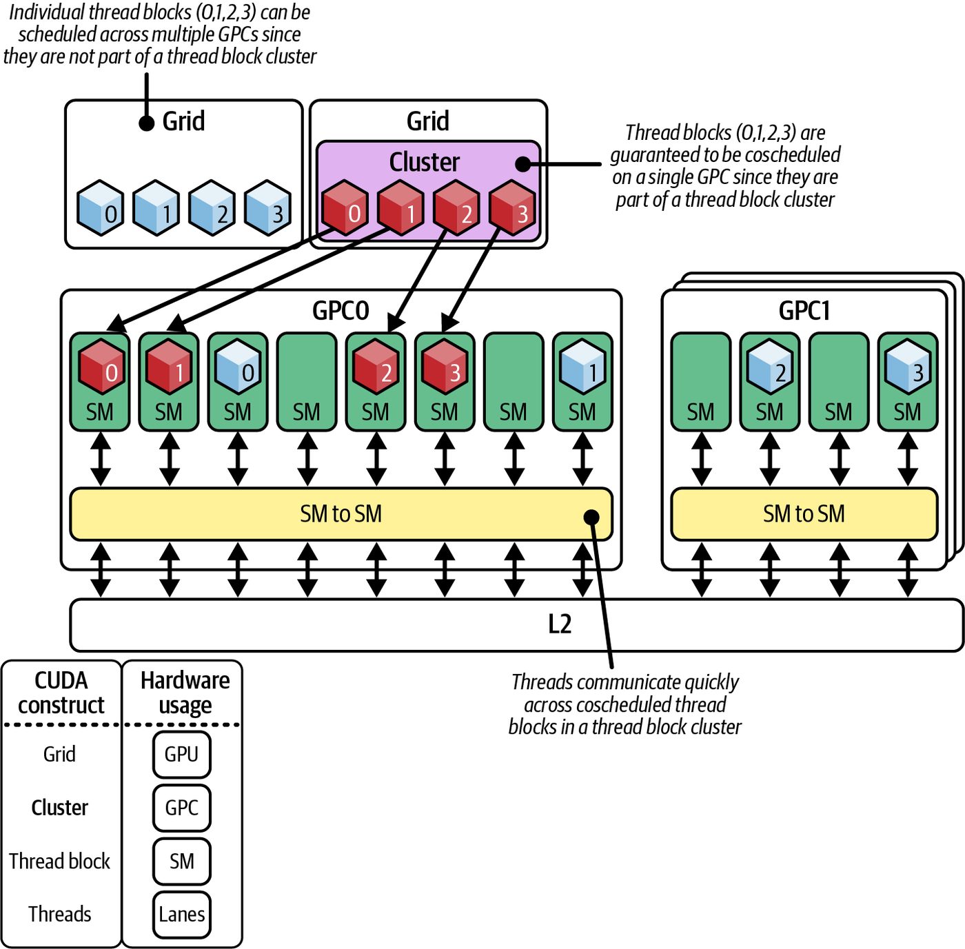
A GPC is a collection of nearby SMs. The GPU schedules thread blocks onto GPCs similar to how it schedules threads of a thread block onto the same SM.
                There are actually multiple GPC “partitions” on multidie modules
                like the NVIDIA Blackwell B200/300 and GB200/300—one GPC
                partition per die. Since Blackwell is a two-die GPU, it has two GPC
                partitions. Remember that Blackwell’s two GPU dies are linked
                with NV-HBI and present as a single CUDA device with full cache
                coherence across dies. The L2 caches are coherent across dies, as
                well. As such, the dies form a combined logical GPC so the archi‐
                tecture handles the separate GPC partitions for you.
The GPU provides distributed shared memory (DSMEM), discussed in the next sec‐ tion, for the thread block cluster to use across those blocks. It also supports a clusterlevel barrier using the Cluster Group API (cluster.sync()). This cluster-level barrier lets you synchronize only a subset of thread blocks without blocking the entire GPU. Thread block clusters let you launch a cooperative kernel that subdivides the grid into smaller groups of blocks, as shown in Figure 10-11.
Figure 10-11. For these four (2 × 2) thread clusters, each tile of A and B is loaded into two thread blocks simultaneously (source: https://oreil.ly/kEZsv)
Within each group, calling cluster.sync() provides a local barrier. This lets blocks inside a cluster share data through dedicated on-chip resources without monopoliz‐ ing every SM. On modern GPUs, you can use DSMEM, which allows thread block clusters to share a contiguous region of on-chip SRAM. This enables low‐latency communication between blocks in the same cluster with native hardware support.
Thread Block Clusters and Distributed Shared Memory | 403
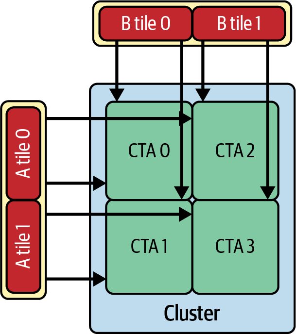
Thread block clusters group a subset of thread blocks and call cluster.sync() within each cluster to synchronize “locally” within just those thread blocks. While threads within a thread block could traditionally cooperate using shared memory, on modern GPUs, they can now collaborate with each other using thread block clusters and DSMEM. Said differently, without thread block clusters, only threads within the same thread block could share data in shared memory. Different thread blocks would have to coordinate using global memory and global barriers (e.g., a grid.sync()), which stalls all threads and limits scalability. And, furthermore, threads in different thread blocks previously could not efficiently share state and synchronize except using either global memory or grid.sync() for coarse-grained, grid-wide synchronization, as described in the previous section. Unfortunately, both global memory and grid.sync() are relatively slow and, as such, can become bottlenecks. Thread block clusters are supported natively by the GPU hardware, including cluster launch control. Cluster launch control is a hardware-level mechanism that launches and schedules persistent thread block clusters. Specifically, it allows a persistent ker‐ nel (and its thread block cluster) to maintain a balanced load of work—even when some of the SMs are occupied. This provides the basis for an efficient warp specializa‐ tion implementation. Using hardware-supported communication and synchronization constructs, thread block clusters can synchronize using cluster-wide barriers in the form of low-level PTX instructions and CUDA intrinsics. As such, blocks in a cluster can perform bar‐ rier synchronization much faster than a full grid synchronization using grid.sync() due to the hardware-supported barrier synchronization between the thread blocks.
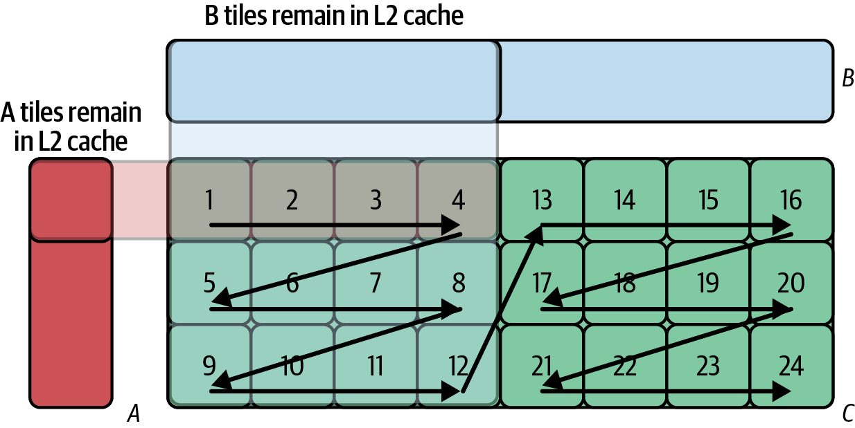
Thread Block Swizzling In a straightforward grid launch, thread blocks process tiles in strict row-major or column-major order. This can cause early blocks to evict data that later blocks will need—resulting in poor reuse and extra memory traffic. Instead, you want tiles A and B within a single wave, which can be read out of L2 cache. To work around this inefficiency, you can use thread block swizzling. Similar to using swizzling to optimize memory access and avoid shared-memory bank conflicts, you can use thread block swizzling to avoid assigning tiles in the inefficient row-major and column-major order, as shown in Figure 10-12.
404 | Chapter 10: Intra-Kernel Pipelining, Warp Specialization, and Cooperative Thread Block Clusters
Figure 10-12. Thread block swizzling to read tiles A and B in a single wave out of L2 cache
Thread block swizzling lets tiles of both A and B matrices, needed by the same wave, stay in L2 for maximum reuse. When applied to persistent and tiled GEMM work‐ loads, this type of swizzling can produce double-digit performance gains by reducing memory misses and bandwidth pressure. Thread-block swizzling is a simple yet pow‐ erful pattern-reordering technique that aligns kernel launch order with cache locality. With hardware support for thread block clusters, a relatively large number of SMs, and improved pipeline scheduling, modern GPUs can host large persistent kernels with a sophisticated warp specialization pipeline to optimize kernel performance. In short, thread block clusters build on the cooperative groups model by allowing a subset of blocks to synchronize and share state without locking out the entire GPU. This lets you build multistage, fine-grained pipelines inside one launch without lock‐ ing out the rest of the device. This leaves the remaining SMs free to perform inde‐ pendent work. Within thread block clusters, there are two key mechanisms to share state between thread blocks: DSMEM and scratch memory. Let’s describe these next.
Distributed Shared Memory Distributed shared memory (DSMEM) extends the concept of __shared__ memory beyond a single thread block to span an entire thread block cluster. In a traditional kernel, each thread block has its own private __shared__ region and is inaccessible to other thread blocks. With DSMEM, however, multiple blocks in the same cluster can read/write into a shared memory space that logically combines all of their local __shared__ regions. In
Thread Block Clusters and Distributed Shared Memory | 405
effect, the cluster’s shared memory is stitched together into one distributed on-chip buffer. By keeping interblock data inside on-chip memory, DSMEM significantly increases effective arithmetic intensity since blocks can exchange intermediate results or per‐ form reductions without round-tripping to global memory. This is especially valuable when a dataset is too large for a single block’s shared memory. Instead of falling back to global loads and stores, you launch a thread block cluster whose blocks each work on a portion of the data, then synchronize and share using DSMEM. All communication happens at SM-to-SM speed, which avoids expensive HBM traffic. In short, DSMEM is a faster, more structured alternative to using global memory for block-to-block communication. But its scope is limited to the blocks in the same clus‐ ter. DSMEM is ideal for persistent kernels that require frequent, low-latency inter‐ block coordination, attention mechanisms, or other multistage algorithms in LLMs in which every block must exchange intermediate state before proceeding—as well as any workload that benefits from keeping interim results on-chip rather than writing back to and reloading from global memory.
                     The portable maximum cluster size is 8 blocks. Some GPUs
                     support larger non-portable cluster sizes (e.g., up to 16 CTAs) when
                     explicitly enabled with the cudaFuncAttributeNonPortableCluster
                     SizeAllowed attribute. This increases your DSMEM footprint at the
                     cost of occupying more SMs in the cluster.
Scratch Memory Scratch memory is the low-level hardware infrastructure that underpins DSMEM and thread block cluster synchronization, whereas DSMEM is the shared data buffer that is implicitly visible to your CUDA code, scratch memory is a separate on-chip SRAM region used by the GPU to track coordination metadata such as barrier state, group progress, and access flags for DSMEM. You do not access scratch memory directly from your kernels. Instead, the GPU man‐ ages it automatically. When you launch a thread block cluster, the hardware allocates a portion of scratch memory to maintain cluster-wide barrier counters (cluster .sync() state), track which blocks have arrived at DSMEM operations or synchroni‐ zation points, and coordinate safe access to the distributed shared regions across SMs. Because scratch memory is optimized for these metadata operations, it enables cluster-level barriers and DSMEM accesses to complete very quickly. If the metadata size exceeds available scratch SRAM for very large clusters or complex
406 | Chapter 10: Intra-Kernel Pipelining, Warp Specialization, and Cooperative Thread Block Clusters
synchronization patterns, the GPU transparently spills some state into local memory, which is backed by L1/L2 caches. This spill ensures correctness while still preserving as much on-chip efficiency as possible. In short, DSMEM is the abstraction you use to share data between blocks and scratch memory in the behind-the-scenes facility that makes those DSMEM operations fast and scalable. Together, they allow a thread block cluster to behave like a single logical unit that breaks the traditional barrier between thread blocks. This improves perfor‐ mance for workloads that need tightly coordinated parallelism across multiple thread blocks.
Launching a Thread Block Cluster
Let’s illustrate how to use thread block clusters in practice. First, we need to launch a
kernel with a cluster dimension that we haven’t used before.
In CUDA, this is done with an extended launch API that allows specifying the cluster
size. For example, if we want clusters of two blocks, also called a thread block pair, or
CTA pair, we can configure a special launch attribute, as shown here:
    // Host code: launch a kernel with thread block clusters of size 2
    cudaLaunchConfig_t config{};
    config.gridDim = dim3(128, 1, 1);
    config.blockDim = dim3(256, 1, 1);
    config.dynamicSmemBytes = 0;
    cudaLaunchAttribute attr{};
    attr.id = cudaLaunchAttributeClusterDimension;
    attr.val.clusterDim.x = 2;
    attr.val.clusterDim.y = 1;
    attr.val.clusterDim.z = 1;
    config.attrs = &attr;
    config.numAttrs = 1;
    // Allow non-portable cluster sizes if you intend to use > 8 later
    cudaFuncSetAttribute(MyClusterKernel,
                         cudaFuncAttributeNonPortableClusterSizeAllowed,
                         1);
cudaLaunchKernelEx(&config, MyClusterKernel, args, nullptr);
In this host code, we use cudaLaunchKernelEx to launch MyClusterKernel with clus‐ ters of 2 thread blocks (so 64 clusters total since 128 blocks ÷ 2 per cluster). The clusterDim is set to 2, meaning each cluster will contain 2 thread blocks. This replaces the traditional <<<gridDim, blockDim>>> syntax for cases where we want cluster-cooperative kernels. Under the hood, the CUDA runtime ensures those paired blocks are scheduled such that they can communicate with DSMEM.
Thread Block Clusters and Distributed Shared Memory | 407
                     Remember that each thread block cluster needs to physically fit
                     into the SMs and resources that you specify. The portable maxi‐
                     mum cluster dimension is 8 thread blocks. To launch 16 on sup‐
                     ported Blackwell parts, you must enable the non-portable attribute
                     and size blocks so the cluster stays resident on the SMs. Keep this
                     in mind when sizing your thread block clusters.
Coordinating Thread Block Clusters with Cooperative Groups API To coordinate work across multiple thread blocks in a cluster, you first obtain a han‐ dle to that group of blocks using cooperative_groups::this_cluster(). This clus‐ ter handle lets you perform hardware‐accelerated cluster-wide barriers—and directly access another block’s shared memory. This all happens without leaving the kernel or resorting to global‐memory flags. Here is an example kernel that sums a local value from each thread block into thread block 0’s shared memory: #include <cuda_runtime.h> #include <cooperative_groups.h> namespace cg = cooperative_groups;
      __global__ void MyClusterKernel(/* args */) {
          // 1. Form a cluster group for all thread blocks in this thread block cluster
          cg::cluster_group cluster = cg::this_cluster();
           // 2. Allocate the same extern shared buffer in each block
           extern __shared__ int shared_buffer[];
           // 3. Each block learns its rank and the total cluster size
           int clusterRank = cluster.block_rank();
           int clusterSize = cluster.num_blocks();
           // 4. Initialize this block’s portion of shared memory (a simple local sum)
           int localSum = threadIdx.x;
           shared_buffer[threadIdx.x] = localSum;
           // 5. Barrier across all blocks in the cluster; no block proceeds until
           //    every block reaches this point and has written its shared_buffer.
           cluster.sync();
           // 6. Map a pointer to block 0’s shared_buffer so block can write into it
           // Pointers returned by cluster.map_shared_rank
           // refer to the remote CTA’s shared memory
           // and support remote atomics
           // and memory operations within
           // the cluster
           // Pair updates with cluster.sync at well defined point
           int* remote_buffer = cluster.map_shared_rank(shared_buffer, 0);
408 | Chapter 10: Intra-Kernel Pipelining, Warp Specialization, and Cooperative Thread Block Clusters
        if (clusterRank != 0) {
            // 7. Nonzero blocks atomically add their local shared_buffer[0] into
            //    rank 0’s buffer. This atomicAdd is routed on‐chip over DSMEM
            //    (not through DRAM.)
            atomicAdd(&remote_buffer[0], shared_buffer[0]);
        }
        // 8. Another cluster‐wide barrier ensures all atomic adds have completed
        cluster.sync();
        // 9. Finally, block 0 (rank 0, thread 0) can read the combined result
        if (clusterRank == 0 && threadIdx.x == 0) {
            printf("Combined sum in cluster[0]: %d\n", shared_buffer[0]);
        }
    }
Here, we obtain a cluster handle by calling cg::this_cluster(). This returns a cluster_group object that represents exactly those blocks launched together as one thread block cluster. The runtime guarantees that every thread block in this cluster group is resident simultaneously—otherwise, the launch will fail. A uniform shared memory allocation is implicitly provided. Each block in the cluster must declare the same size for extern __shared__ int shared_buffer[]. The DSMEM hardware will then logically combine each block’s shared memory into one virtual address space. And because all blocks reserve the same shared_buffer size, a pointer to the buffer of thread block 0, or rank 0, will coordinate properly across SMs.
               When using thread block clusters, make sure to organize each
               thread block’s DSMEM accesses just like global‐memory coalesc‐
               ing. In other words, have each warp read or write contiguous, 32-
               byte-aligned sectors. That way, the hardware can route cluster-wide
               DSMEM transfers without bank conflicts or unexpected serializa‐
               tion. In practice, lay out your tile data so that the warp i in thread
               block j always touches a unique, aligned range. This will avoid
               memory bank contention and keep DSMEM data transfers per‐
               forming at full speed.
In the previous example code, we also see that cluster.sync() is used as a clusterwide barrier across thread blocks in the cluster. Unlike __syncthreads(), which only synchronizes threads within a single block, cluster.sync() synchronizes all threads in every block of this cluster. This barrier is implemented in hardware and generally has lower latency than a gridlevel synchronization, because it coordinates only the blocks in the cluster. This means you can synchronize blocks frequently with minimal impact—as long as they are within a cluster.
Thread Block Clusters and Distributed Shared Memory | 409
And there is no risk of deadlock caused by missing blocks since CUDA enforces that the grid launches properly and fits on the GPU. As such, there is no scenario in which some blocks reach the barrier and then hang forever waiting for “missing” blocks that never started. All blocks are already present, so the barrier completes cleanly once every block calls it. In the previous code block, you see that cross‐block shared memory access happens using map_shared_rank(). After the first barrier, every block’s shared_buffer[] is initialized. To get a pointer into block 0’s shared memory, the other blocks call int* remote_buffer = cluster.map_shared_rank(shared_buffer, 0), which specifies the thread block id (0) in the cluster. The GPU hardware automatically translates that pointer so any load or store goes over the on‐chip DSMEM network rather than out to global DRAM. As such, any write operation into remote_buffer—either an atomic or regular write—will update block 0’s shared memory directly on‐chip. It’s worth highlighting that the perfor‐ mance characteristics of remote DSMEM accesses differ from local shared memory. Remote loads and stores benefit from coalesced, aligned 32-byte segments. For instance, in the previous code block, when blocks 1...n need to add their local val‐ ues into block ID 0’s shared buffer, they call atomicAdd(&remote_buffer[0], shared_buffer[0]). And because remote_buffer was obtained with clus ter.map_shared_rank(), the atomicAdd goes directly into block 0’s SMEM over the on‐chip DSMEM network. In other words, there is no round trip to DRAM or L2 cache. Every write happens at on‐chip speeds. In the previous code example, you see that once all blocks have performed their atom icAdd, a second cluster.sync() ensures that block 0 sees the complete sum in its own shared_buffer[0] before proceeding. In short, cooperative_groups::this_cluster() plus cluster.sync() and cluster .map_shared_rank() give you a simple, efficient way to synchronize and share data across multiple thread blocks in a thread block cluster. All of these operations occur on‐chip, avoid global‐memory round trips, and enable fine‐grained cooperation among blocks. This combination of thread block clusters and DSMEM provides much higher performance than any global‐memory fallback or manual atomic‐flag approach.
Thread Block Pair With modern NVIDIA, GPUs let you coschedule exactly two thread blocks in a clus‐ ter, or a thread block pair (aka CTA pair), across SMs within a single GPC. By group‐ ing thread blocks in a cluster (e.g., a 2-block cluster, as shown in Figure 10-13), kernels that share data can use TMA to move tiles into each block’s shared memory.
410 | Chapter 10: Intra-Kernel Pipelining, Warp Specialization, and Cooperative Thread Block Clusters
Figure 10-13. Thread block pair combines two thread blocks
A single thread block might lack the registers or shared‐memory capacity to process a very large tile (for example, a 256 × 256 matrix subtile) by itself. By pairing two thread blocks on nearby SMs within a GPC and using DSMEM, those two blocks can split the work on one large tile yet share data through a unified shared‐memory region, as shown in Figure 10-14.
Figure 10-14. Thread block pair (aka CTA pair) loading tiles as operands for an A * B matrix multiply (source: https://oreil.ly/kEZsv)
Here, each thread block in the pair can load a fraction of the operand tile (e.g., 128 × 16) into its on-chip SMEM for the matrix multiply. In addition, each thread block holds part of the accumulator (e.g., 128 × 256) in Tensor Memory (TMEM). This
Thread Block Clusters and Distributed Shared Memory | 411
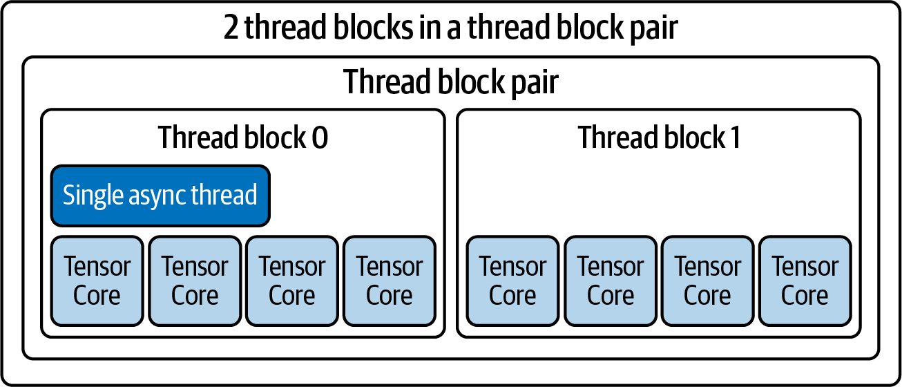
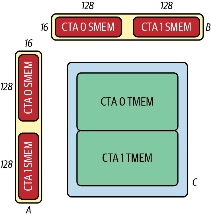
allows the two thread blocks in the CTA pair to collaborate on a single tile, as shown in Figure 10-15.
Figure 10-15. Thread block pair with Tensor Cores and TMEM
Thread block pairs allow larger matrix multiplies that span two physical SMs. Using a pair of thread blocks effectively doubles the tile size since each SM handles half of the tile’s data. The SM hardware shares operand data between the SMs using DSMEM. DSMEM reduces duplicate loads, improves data reuse, and increases arithmetic intensity. Figure 10-16 shows this data sharing between SMs in a thread block cluster using DSMEM.
Figure 10-16. Sharing data between SMs in a thread block cluster using DSMEM
412 | Chapter 10: Intra-Kernel Pipelining, Warp Specialization, and Cooperative Thread Block Clusters
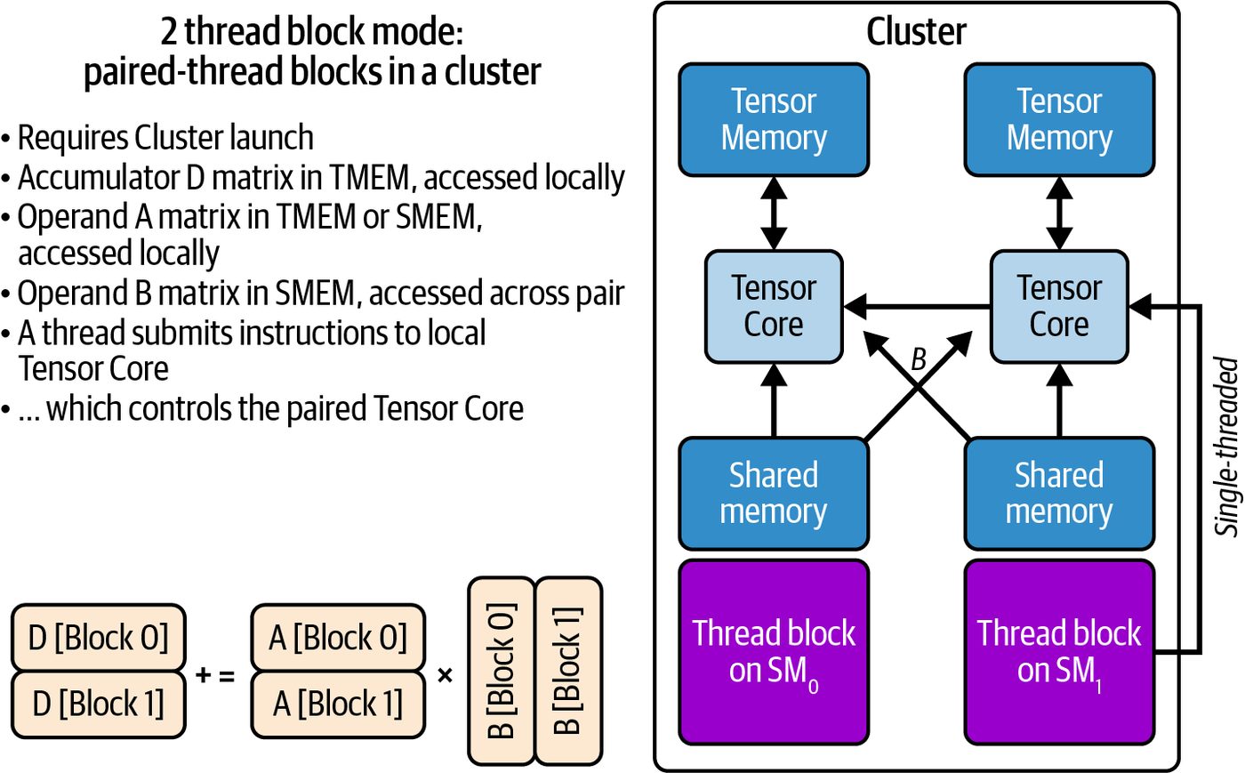
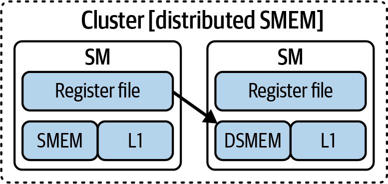
CUDA provides enhanced multicast barrier and synchronization primitives for these multi-SM operations. The pair synchronizes with each other using the lightweight cluster.sync() call. This way, when one SM finishes using a tile, the adjacent SM in the CTA pair can consume it. Each tile is fed into the pair of thread blocks without redundant global-memory transactions. This better occupies otherwise idle registers, shared-memory banks, and Tensor Cores. And a thread block pair achieves higher Tensor Core utilization by doubling the threads and shared memory available for one tile. Any boost in performance will happen transparently. From a programmer’s perspec‐ tive, you simply launch a cluster of two blocks and treat it as one large thread block split across two thread blocks. In CUTLASS, for instance, this is exposed as a 2-SM UMMA (Unified MMA) GEMM operation that uses DSMEM and cluster barriers for inter-CTA data sharing. You simply request two SMs for a single GEMM tile, and CUTLASS handles the cluster launch, DSMEM setup, and interthread block synchro‐ nization automatically. If you request a tile size that a single thread block can’t handle (say, 128 × 128 for FP16 Tensor Core operations), CUTLASS will automatically allocate two thread blocks as a pair. The SMs split the work and rely on DSMEM + cluster.sync() under the hood to share the tile. This way, you can do pairwise overlapping of UMMA operations with DSMEM. In short, thread block pairs and DSMEM provide parallelism in the form of multi-SM cooperation. They provide fast, on-chip data sharing and synchronization across thread blocks. This eliminates many scenarios that previously required globalmemory handoffs or additional kernel launches. This benefits many multithread block algorithms and simplifies their implementation.
Reducing Global Memory Traffic with Thread Block Clusters From a performance perspective, DSMEM can significantly cut down redundant global‐memory traffic and enable higher effective bandwidth. For instance, in a tiled GEMM where multiple thread blocks within a cluster share chunks of the A or B matrix, one block can load a tile from global memory and multicast the tile to other blocks in the cluster using the TMA. The TMA engine supports a multicast copy mode that feeds directly into DSMEM when thread blocks belong to the same cluster. A single TMA transfer from global memory can place data into each participating block’s shared memory simultane‐ ously. This avoids redundant DRAM fetches.
Reducing Global Memory Traffic with Thread Block Clusters | 413
With TMA multicast, the GPU ensures that L2‐cached data is broadcast into the shared memory of each cluster member (thread block) in one pass. As a result, you avoid repeated global‐memory loads of the same tile. This improves bandwidth utilization and shrinks DRAM traffic—especially when many blocks need the same input, as shown in Figure 10-17.
Figure 10-17. For these four (2 × 2) thread clusters, each tile is loaded once and multi‐ cast into the shared memory of all CTAs in each cluster (source: https://oreil.ly/kEZsv)
Here, the TMA engine performs a single multicast from global memory into DSMEM, broadcasting the tile to every thread block’s SMEM in the cluster and elimi‐ nating redundant DRAM reads. TMA multicast is configured through a tensor-map descriptor and issued as cp.async.bulk.tensor targeting shared::cluster. Fortu‐ nately, higher-level libraries like CUTLASS/cuTe and Triton generate these multicast operations, tensor-map descriptors, and bulk tensor copies for you. Specifically, these libraries can issue the relevant PTX instructions including cp.async.bulk.tensor with a tensor-map operand. They can issue PTX instructions that target shared::cluster for multicast. In these cases, the hardware delivers the tile to each thread block’s SMEM. Another common use case is multiblock reductions or scans. Instead of having each block write out its partial sum or scan result to global memory and then launching a separate kernel to combine them, thread blocks in a thread block cluster can write their partial results into DSMEM. Within that same cluster, you can perform a fast on‐chip reduction or prefix‐sum across these partial results using shared memory and a cluster‐level barrier, clus ter.sync(). Only the final result needs to go to global memory. This greatly reduces global memory reads and writes.
414 | Chapter 10: Intra-Kernel Pipelining, Warp Specialization, and Cooperative Thread Block Clusters
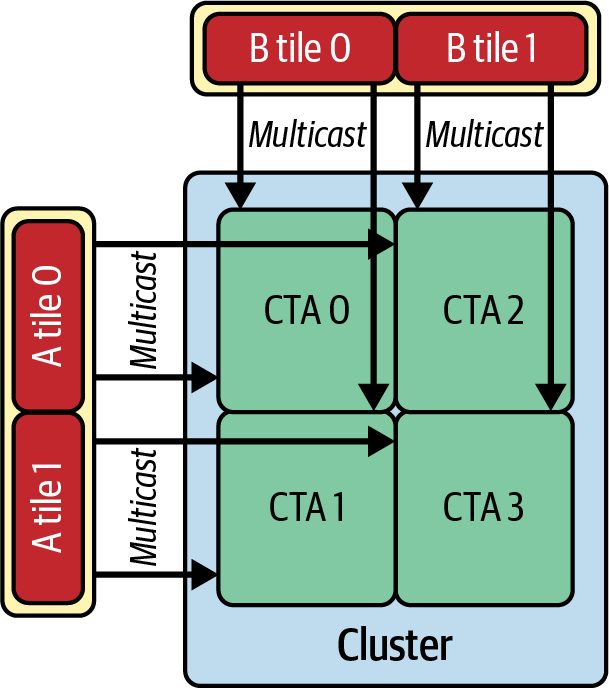
By combining thread block clusters, DSMEM, and TMA multicast, you can build multistage, fine‐grained pipelines that keep most data exchanges on‐chip. Whether you are sharing tiles for GEMM, accumulating partial sums for a reduction, or performing a multiblock scan, these mechanisms let you minimize HBM round trips and maximize arithmetic intensity.
                         A block scoped cuda::pipeline does not synchronize other
                         blocks; cluster wide distribution uses TMA multicast or DSMEM
                         with cluster.sync.
Consider two thread blocks, CTA 0 and CTA 1, that both need the same tile of matrix A. Without DSMEM, each CTA issues its own global‐memory load, which wastes DRAM bandwidth by fetching the identical data twice. With DSMEM, however, CTA 0 loads the tile once into its shared memory and then multicasts it over the on-chip DSMEM network so that CTA 1 can read it directly from shared memory. If more than two CTAs form a cluster, the same tile will be shared across all thread blocks in the cluster, but this still requires only one global HBM load. Table 10-4 shows a comparison using a cluster of two thread blocks versus two independent thread blocks.
Table 10-4. Performance impact of DSMEM on a two-block workload Metric Two independent CTAs (no DSMEM) CTA pair with DSMEM (cluster of 2) Global load transactions 2× (each thread block loads tile) 1× (tile loaded once) L2 cache hit rate 50% 85% Inter-CTA data reuse N/A (no reuse) Significant (tile reused by CTA 1) Effective DRAM BW per CTA 300 GB/s 50% less 150 GB/s Kernel time (relative) 1.0× 0.6× (40% speedup)
Here, we see a 40% speedup in kernel execution when using a thread block pair (aka CTA pair) with DSMEM. This is consistent with the bandwidth savings as well. The DRAM bandwidth per thread block drops by 50% from 300 GB/s to 150 GB/s since each tile is fetched only once. The L2 hit rate jumps from 50% to 85% since the TMA hardware is performing a multicast copy on-chip—and therefore avoiding multiple loads from global memory. In short, by multicasting shared data, thread block clusters allow multiple blocks to reuse data at on-chip speeds. This leads to substantial speedups for memory-bound workloads.
Reducing Global Memory Traffic with Thread Block Clusters | 415
It’s important to note that both DSMEM and L2 operate in parallel. This provides two “lanes” for interblock data sharing. This dual‐path design combines DSMEM’s ultra‐ fast cluster-wide communication with L2’s broader caching coverage. In other words, DSMEM access is bypassing the L2 cache for cluster-local addresses. Instead, DSMEM uses the dedicated SM-to-SM network, as shown in Figure 10-18.
Figure 10-18. DSMEM uses an SM-to-SM thread block cluster-local network between two thread block clusters for its data exchange
Remote DSMEM accesses are routed using the thread block cluster interconnect and are distinct from global-memory traffic. For example, when a thread block pulls a tile using DSMEM, it uses low-latency shared‐memory transfers. This ensures that inter‐ thread block data sharing in a thread block cluster is as fast as on-chip shared memory. If a tile is not present in DSMEM, it must be fetched from global memory (following the normal cache hierarchy that may hit in L2, for example). This way, if a tile has already been evicted from DSMEM, for instance, the thread block can still retrieve the tile data from the L2 cache instead of going all the way back to global DRAM. As a result, memory stalls are rare, occupancy remains high, and overall execution runs significantly faster than the unoptimized, two-independent-thread-blocks, nonDSMEM implementation.
Designing Efficient Algorithms with Thread Block Clusters Thread block clusters enable new strategies for parallelizing workloads that previ‐ ously required global memory communication or multiple kernel launches. For example, imagine a large matrix multiplication in which the output tile is too large to be handled by a single thread block due to shared memory limits. In the past, you might split the work across two thread blocks, but then each block would have to exchange partial results with global memory, which is relatively slow and inefficient. Otherwise, you’d have to launch a separate reduction kernel to com‐ bine the outputs of the two thread blocks. With thread block clusters and DSMEM, those two blocks can form a cluster and directly share a joint region of on-chip shared memory to seamlessly combine their results using hardware-supported primitives. The DSMEM hardware allows an SM to
416 | Chapter 10: Intra-Kernel Pipelining, Warp Specialization, and Cooperative Thread Block Clusters
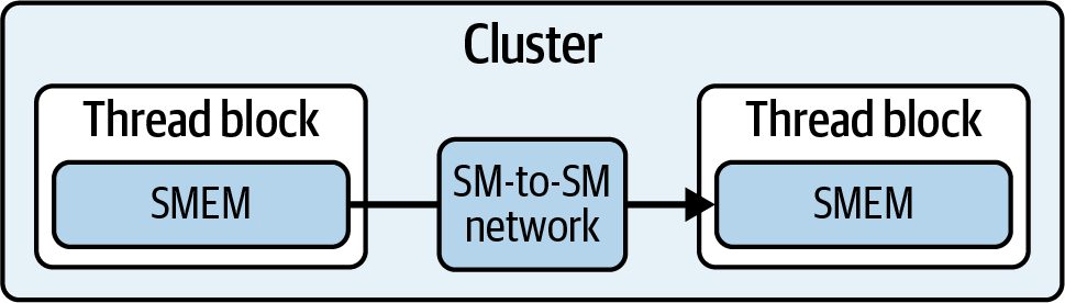
perform loads/stores/atomics to another SM’s shared memory through a fast network. It’s important to carefully design algorithms to use thread block clusters effectively. Synchronization overhead is low, but it is still nonzero. Performing very fine-grained data sharing might not pay off. Thread block cluster barriers work like warp‐level intrinsics (e.g., __shfl_sync()), introduced in Chapter 7, in that every participant must arrive at the synchronization point together. When you call cluster.sync(), all thread blocks in the cluster must reach that line before any block can continue. If one block finishes its work early, it simply waits. If a block never reaches the bar‐ rier, because its threads took a different branch, for instance, the entire cluster will deadlock. In other words, just as warp intrinsics demand that all threads in a warp execute the same instruction path to avoid divergence, thread block clusters demand that all blocks follow the same control flow up to each cluster.sync() call. Because of this lockstep requirement, fine‐grained data sharing between blocks must be balanced against the overhead and risk of deadlock. Synchronization itself is inex‐ pensive when done correctly, but if even one block bypasses or delays reaching a clus ter.sync(), performance may be impacted—or, even worse, the kernel might hang. You should structure code such that every block arrives at each barrier in unison— just as every thread in a warp must arrive at the barrier with warp‐level intrinsics. This is essential to take full advantage of the thread block clusters’ low‐latency, on‐ chip communication without falling into deadlocks. Typically, thread block clusters perform the best when each block has a sizable amount of work that can run independently until a synchronization or data exchange point is needed. Once the synchronization happens and the data is transferred onchip, the thread blocks can continue processing. Thread block clusters are especially effective for block‐sparse matrix operations— common in sparse attention, model pruning, and compression in LLMs. In these cases, the blocks process different nonzero regions and share their boundary data. Thread block clusters are also useful for multiphase reductions such as the softmax and normalization steps in transformer layers. These require a final combine step using the partial results of each thread block in the thread block cluster. More generally, large GEMMs benefit from thread block clusters when they exceed the resources of a single block. GEMMs, of course, are central to the transformer attention and multilayer perceptron (MLP) layers and embedding lookups common in modern LLMs.
Designing Efficient Algorithms with Thread Block Clusters | 417
Larger cluster sizes can reduce overall occupancy, however. For instance, a cluster of 16 blocks might monopolize 16 SMs for one task. This could leave fewer SMs for other tasks needed by that kernel launch. It’s recommended to start with small clus‐ ters, twoor four-thread block clusters, unless a bigger cluster is needed for special cases. As always, you should profile with your specific workload to confirm that shar‐ ing on-chip resources across thread block clusters outweighs the potential loss of parallelism.
                     When using cluster launches, verify active blocks and cluster resi‐
                     dency with Nsight Compute launch statistics and the standard
                     occupancy APIs, such as cudaOccupancyMaxActiveBlocksPer
                     Multiprocessor. For nonportable cluster sizes, set cudaFuncAttri
                     buteNonPortableClusterSizeAllowed (or pass cudaLaunchAttrib
                     uteNonPortableClusterSizeAllowed using cudaLaunchKernelEx
                     attributes). Otherwise the launch may fail or measure low
                     occupancy.
Warp Specialization with Thread Block Clusters Let’s now revisit warp specialization using a thread block cluster with the CUDA Pipeline API. We use a thread-block scoped pipeline as the cluster leader to stage the copies and perform cluster-wide barriers with DSMEM. This way, every block in the cluster consumes the same input tiles without reloading them from global memory. Roles are assigned per warp inside each block. The leader block’s loader warp per‐ forms the cooperative copies into its shared memory once per tile. After a clusterwide barrier publishes those tiles, every block uses a compute warp to read the leader’s tiles through DSMEM and compute a disjoint band of rows. A storer warp in each block writes that band back to global memory. The block-scoped pipeline is used only by the leader for the asynchronous copies. Other blocks do not wait on that pipeline. Here is the code: // Warp specialization across a thread-block cluster // using DSMEM and a block-scoped pipeline
      #include <cuda/pipeline>
      #include <cooperative_groups.h>
      #include <algorithm>
      namespace cg = cooperative_groups;
      #define TILE_SIZE 128
      #define TILE_ELEMS (TILE_SIZE * TILE_SIZE)
      // Compute a band of rows of the TILE_SIZE×TILE_SIZE product from DSMEM sources.
      // Each lane processes rows [row_begin, row_end) in a 32-way striped loop.
      __device__ void compute_rows_from_ds(const float* __restrict__ A_src,
418 | Chapter 10: Intra-Kernel Pipelining, Warp Specialization, and Cooperative Thread Block Clusters
                                     const float* __restrict__ B_src,
                                     float* __restrict__ C_dst,
                                     int row_begin, int row_end,
                                     int lane_id) {
    for (int row = row_begin + lane_id; row < row_end; row += warpSize) {
        for (int col = 0; col < TILE_SIZE; ++col) {
            float acc = 0.0f;
            #pragma unroll
            for (int k = 0; k < TILE_SIZE; ++k) {
                acc += A_src[row * TILE_SIZE + k] * B_src[k * TILE_SIZE + col];
            }
            C_dst[row * TILE_SIZE + col] = acc;
        }
    }
}
extern "C"
__global__ void warp_specialized_cluster_pipeline(
    const float* __restrict__ A_global,
    const float* __restrict__ B_global,
    float* __restrict__ C_global,
    int numTiles) {
    thread_block cta = this_thread_block();
    cluster_group cluster = this_cluster();
    extern __shared__ float shared_mem[];
    float* A_tile_local = shared_mem;
    float* B_tile_local = A_tile_local + TILE_ELEMS;
    float* C_tile_local = B_tile_local + TILE_ELEMS;
    // Block-scoped pipeline used only by the cluster leader
    // to stage asynchronous copies
    __shared__
    cuda::pipeline_shared_state<cuda::thread_scope_block, 2> pipe_state;
    auto pipe = cuda::make_pipeline(cta, &pipe_state);
    const int lane_id = threadIdx.x & 31;
    const int warp_id = threadIdx.x >> 5;
    const int cluster_rank     = cluster.block_rank();
    const dim3 cluster_dims    = cluster.dim_blocks();
    const int blocks_in_cluster = cluster_dims.x * cluster_dims.y *
                                  cluster_dims.z;
    // 1D cluster arrangement along x;
    // each iteration processes one tile per cluster
    auto loader = cooperative_groups::tiled_partition<32>(cta);
    for (int tile = blockIdx.x / cluster_dims.x; tile < numTiles;
         tile += gridDim.x / cluster_dims.x) {
        const size_t offset = static_cast<size_t>(tile) * TILE_ELEMS;
// Leader block’s loader warp stages A and B once for the entire cluster
Warp Specialization with Thread Block Clusters | 419
              if (cluster_rank == 0 && warp_id == 0) {
                  pipe.producer_acquire();
                  cuda::memcpy_async(loader, A_tile, A_global + offset,
                                     cuda::aligned_size_t<32>{TILE_ELEMS*sizeof(float)},
                                     pipe);
                  cuda::memcpy_async(loader, B_tile, B_global + offset,
                                     cuda::aligned_size_t<32>{TILE_ELEMS*sizeof(float)},
                                     pipe);
                  pipe.producer_commit();
                  // Make loads visible to leader CTA before publishing cluster-wide
                  // wait for committed stage before publishin
      pipe.consumer_wait();
                  pipe.consumer_release();
              }
                // Publish the leader’s tiles to every block via DSMEM
                cluster.sync();
                const float* A_src = cluster.map_shared_rank(A_tile_local, 0);
                const float* B_src = cluster.map_shared_rank(B_tile_local, 0);
                // Divide rows among blocks in the cluster
                const int rows_per_block = (TILE_SIZE + blocks_in_cluster - 1)
                                           / blocks_in_cluster;
                const int row_begin = std::min(cluster_rank * rows_per_block, TILE_SIZE);
                const int row_end   = std::min(row_begin + rows_per_block, TILE_SIZE);
                // Compute warp produces block’s band of rows into local shared memory
                if (warp_id == 1) {
                    pipe.producer_acquire();
                    compute_rows_from_ds(A_src, B_src, C_tile_local, row_begin, row_end,
                                         lane_id);
                    pipe.producer_commit(); // publish C_tile_local
                }
                // Storer warp writes this block’s rows back to global memory
                if (warp_id == 2) {
                    pipe.consumer_wait(); // observe C_tile_local
                    for (int row = row_begin + lane_id; row < row_end; row += warpSize) {
                        for (int col = 0; col < TILE_SIZE; ++col) {
                            C_global[offset + row * TILE_SIZE + col] =
                                C_tile_local[row * TILE_SIZE + col];
                        }
                    }
                    pipe.consumer_release();
                }
                // All blocks finish this tile before the leader reuses its buffers
                cluster.sync();
           }
           // dynamic shared memory size: 3 * TILE_ELEMS * sizeof(float)
      }
420 | Chapter 10: Intra-Kernel Pipelining, Warp Specialization, and Cooperative Thread Block Clusters
Here, the leader performs one pair of cooperative copies of each tile into its shared memory using a block-scoped pipeline. The cluster-wide barrier makes the data visi‐ ble to all cluster members through DSMEM. This “copy once, share through DSMEM” pattern shares the leader’s tiles using DSMEM and map_shared_rank following a cluster barrier. It does not perform a TMA multicast as we covered previously with tensor-map descriptors, cp.async.bulk.tensor, and shared::cluster. This is an important distinction to understand as, without the cluster.sync() in the DSMEM pattern, followers can read stale leader SMEM data. As such, cluster.sync() is required before map_shared_rank().
               The following should help you choose TMA multicast versus
               DSMEM sharing: If tile reuse per block is high (e.g., each block
               touches the same tile many times) or the cluster size (C) is large
               (8-16 CTAs), TMA multicast usually wins since this pattern writes
               once, then reads locally many times. If SMEM is tight (e.g., large
               tiles) or cluster size (C) is small (2-4 CTAs) and each follower
               touches the tile once, DSMEM sharing is usually the better option
               since it uses a smaller footprint.
Every block computes a distinct band of rows directly from the leader’s shared mem‐ ory by using map_shared_rank and writes its results to global memory. This removes duplicate global loads across the cluster and keeps the overlap advantages of a pipe‐ line at the points where it matters. The leader block’s loader warp calls producer_commit() to publish its local stage to that block. Other blocks do not wait on the leader’s pipeline. Instead, they observe the leader’s tiles after the cluster wide barrier and then read from distributed shared memory. This allows tile loading, computing, and storing to interleave across multiple thread blocks, which drives the SMs to even higher utilization. Table 10-5 compares the single-block warp-specialized kernel with the thread-block-clustered (multiblock) warp-specialized kernel presented in this section.
Warp Specialization with Thread Block Clusters | 421
Table 10-5. Comparison of naive tiling, two‐stage double buffering, warp‐specialized, and thread block cluster pipeline kernels. Metric Naive Two-stage, doubleWarp-specialized Thread block cluster tiling buffered (double_ (warp_special pipeline (warp_special buffer_pipeline) ized_pipeline) ized_cluster_ pipeline) Kernel execution 41.3 ms 20.5 ms (+2.01× faster 18.4 ms (+10.2% speedup 17.2 ms (+6.5% speedup time versus naive) versus two-stage) versus warp-specialized) Warp execution 68% 92% (+24% versus 96% (+4% versus two-stage) 97% (+1% versus warpefficiency naive) specialized) Warp state stall % High Low Minimal Minimal (further reduced) (for shared memory and barrier waits) L2 throughput 80 GB/s 155 GB/s (+94% versus 165 GB/s (+6.45% versus two170 GB/s (+3% versus warpnaive) stage) specialized) Throughput Scales up Scales to ~6 warps/SM Scales nearly linearly to SM Scales fully across thread scalability to 2–3 warp limit (64 resident warps blocks until they are warps/SM per SM on Blackwell) constrained by SM warp limit of 64 resident warps per SM on Blackwell DRAM read Poor Great overlap Excellent overlap Excellent overlap (even throughput versus overlap under thread block handoff) kernel duration Instruction count 1.7 B 1.05 B (–38% versus ~1.00 B (–4.76% versus two- ~0.98 B (–2% versus warpnaive) stage) specialized)
Here, we see that the thread block cluster implementation further improves on warp‐ specialized by distributing loader, compute, and storer roles across multiple thread blocks in one cooperative launch. This increases overall SM utilization and reduces both execution time and redundant memory traffic. Specifically, the thread block cluster pipeline kernel implementation (warp_special ized_cluster_pipeline) squeezes out another ~1.2 ms (6.5%) over the singlethread-block, warp-specialized kernel. This is because the thread block cluster version interleaves tile loads, computes, and stores across all thread blocks. SM utilization reaches ~97%, since any idle SM in one thread block can be kept busy by another thread block performing a different pipeline stage. L2 load throughput peaks around 170 GB/s, thanks to better shared-memory reuse and fewer redundant loads. As such, the cluster can avoid duplicate global reads. With DSMEM, the leader block loads a tile once and other blocks read it using map_shared_rank() after cluster.sync() is called. With TMA multicast, a single tensor copy from global can be broadcast directly into each block’s shared memory.
422 | Chapter 10: Intra-Kernel Pipelining, Warp Specialization, and Cooperative Thread Block Clusters
Instruction count drops to ~0.98 B because thread-block-wide pipelining further reduces wasted cycles on redundant global reads. Throughput scalability is also main‐ tained since, as long as you have enough thread blocks and warps, the pipeline can keep them all saturated up to the warps-per-SM hardware limit of your GPU, or 64 warps per SM on Blackwell. Note that both the single thread block and thread block cluster versions of warp spe‐ cialization will eventually hit that same “warps‐per‐SM” ceiling, but they differ in how those warps are fed data and synchronized. This difference translates into a measurable performance advantage for the thread block cluster implementation, as we saw in Table 10-5. Specifically, in the single thread block, warp‐specialized kernel, each thread block allocates exactly three warps: one to load a tile‐sized chunk of A and B into shared memory, one to compute on that chunk, and one to store the results back to global memory. Once those three warps complete their roles, the thread block moves on to its next tile, and the cycle repeats. Even if every SM has three active warps for load, compute, and store, you are not sat‐ urating the warp limit of the SM. Modern GPUs allow up to 64 concurrent warps per SM, and actual residency is limited by registers, shared memory, and blocks per SM. At similar total live warp counts, a single-block warp specialized design and a cooper‐ ative grid can show comparable occupancy, but the memory behavior differs. In a single-block design, each block fetches its own copy of any input tile that it touches. When multiple blocks reuse the same tile at about the same time, the device performs duplicate reads that consume L2 capacity and HBM bandwidth. A thread block cluster changes that pattern. Blocks in the cluster can share data through distributed shared memory and can receive one multicast of a global tile into the shared memory of all blocks in the cluster. Use a block-scoped pipeline in the leader block together with cluster synchronization and map_shared_rank, or config‐ ure for multicast when broadcast from global memory is preferred. This removes duplicate loads within the cluster and reduces pressure on L2 and HBM. A cuda::pipeline is scoped to the creating block. A producer_commit() in one block does not release consumer_wait() in other blocks. To coordinate across blocks in a cluster, first publish data (e.g., into the leader’s shared memory), then use clus ter.sync(). Followers then access the leader’s shared memory with map_shared_rank(). Optional TMA multicast can broadcast from global memory directly into each block’s shared memory.
Warp Specialization with Thread Block Clusters | 423
At this point, every block observes the leader’s tiles through DSMEM (or TMA multi‐ cast) and proceeds. The block-scoped pipeline does not explicitly synchronize other blocks. cluster.sync() and DSMEM semantics provide the cluster-wide visibility. When designed to use TMA multicast and DSMEM efficiently, the thread block clus‐ ter pipeline will fetch each tile exactly once and multicast it into every thread block’s shared memory. This is in contrast to redundantly reloading the data from each thread block. As such, although every SM still cannot exceed its 64-warp limit, the global thread block cluster coordination ensures that those warps spend far less time on duplicate loads and far more time on actual computation. Moreover, in the single thread block version, each block loads its next tile as soon as it finishes computing the current one. If one thread block completes its computation slightly earlier than another, it immediately issues its own load for the next tile—even if that tile is already being loaded by another block. This results in redundant mem‐ ory traffic. However, with the thread block cluster pipeline version, if a compute warp on SM 0 finishes early, it does not fetch its next tile immediately. Instead, it stalls at con sumer_wait() until the global loader—possibly running on SM 7—finishes bringing that tile into shared memory for all thread blocks. In other words, the compute warp waits for the cluster’s single, shared load rather than issuing its own redundant copy. By pausing until the tile is guaranteed available, each SM participating in a thread block cluster avoids spinning idle or performing duplicate loads. This alignment across thread block clusters smooths out variations in load times and keeps every SM’s compute warps busy with data loaded only once per cluster. This improves over‐ all throughput. Consider a problem so large and a grid so full of work that every SM already has loader, compute, and storer warps active under the single-block approach. In that case the raw warp counts and per-SM occupancy can look similar between the two kernels. The cluster version helps when multiple blocks reuse the same input tiles by eliminating duplicate global reads within a cluster and by using cluster-wide synchro‐ nization to align stages. This often produces a modest throughput improvement on reuse-heavy workloads, but the gain depends on tile reuse, alignment, and resource limits. Both designs remain bounded by the same architectural limits, such as resident warps, registers, and shared memory. All of the kernels here use the CUDA pipeline for producer and consumer handoffs without calling a block-wide __syncthreads. The naive tiled kernel does not overlap memory and compute. The two-stage double-buffered pipeline overlaps copies with compute and can significantly reduce time to solution on memory-bound cases.
424 | Chapter 10: Intra-Kernel Pipelining, Warp Specialization, and Cooperative Thread Block Clusters
The warp-specialized pipeline dedicates separate warps to load, compute, and store to avoid implicit full-block waits. The thread block cluster variant shares tiles across blocks in a cluster through distributed shared memory or multicast so that a tile is fetched once per cluster rather than once per block. These patterns improve utiliza‐ tion and reduce redundant memory traffic.
Key Takeaways
The following are key takeaways from this chapter, which is focused on extracting
peak performance on modern GPUs. These will keep kernels from idling on DRAM,
warp schedulers, and global barriers:
Hide latency with pipeline depth
    Use two-stage (cuda::pipeline_shared_state<cuda::thread_scope_block,
    2>) tiling to overlap asynchronous loads with compute and add another stage
    (cuda::pipeline_shared_state<cuda::thread_scope_block, 3>) when com‐
    pute outweighs memory (e.g., modern GPUs like Blackwell.) This will help to
    eliminate idle warps.
Balance workloads with warp specialization
    Assign separate warps to loading, computing, and storing when compute phases
    dominate, ensuring near-peak warp efficiency on modern GPU hardware.
Remove launch overhead with persistent kernels
   Run a single long-lived kernel over a device-side work queue and use
   grid.sync() for multiphase algorithms. This will reduce host-device round trips
   and overall launch costs.
Enable on-chip sharing with thread block clusters and DSMEM
   Group thread blocks (CTAs) into clusters so they share a contiguous on-chip
   buffer. For a cluster-wide broadcast, use cp.async.bulk.tensor with a TMA
   multicast descriptor. Use TMA multicast to broadcast tiles once to every thread
   block. This will boost L2 hit rates and trim DRAM bandwidth.
Pay special attention to barrier semantics
    Both cluster.sync() and grid.sync() require every participating thread block
    to reach the same synchronization point. Mismatched control flow—or an exces‐
    sive cluster size—may lead to deadlock or launch failure.
Profile before tuning
    Use Nsight Compute to identify whether your kernel is memory bound or com‐
    pute bound. If memory bound, start with a two-stage pipeline. If compute
    bound, consider warp specialization or thread block clustering.
Key Takeaways | 425
Verify compiler-generated pipelines before hand-tuning
    Profile and inspect the framework’s generated code from compilers like PyTorch’s
    compiler and NVCC. If the compiled code uses an asynchronous pipeline using
    cuda::memcpy_async, producer_commit(), and consumer_wait(), manual tun‐
    ing likely won’t produce much of a speedup.
Conclusion The techniques discussed in this chapter help to systematically hide latency and remove redundant loads. This keeps the GPU at near-peak utilization for the dura‐ tion of the kernel’s execution. Warp-specialized pipelines overlap load, compute, and store operations. Cooperativegroup barriers (grid.sync() and cluster.sync()) help coordinate multiphase work without host round trips. And persistent kernels loop over a device-side queue to eliminate launch overhead. As always, you should start by profiling. If global-memory stalls dominate, a twostage asynchronous-copy pipeline like double buffer usually suffices. If compute warps still stall, switch to a multistage warp-specialized pipeline such that loader, compute, and storer warps can operate with minimal contention. The only conten‐ tion would be at the memory subsystem.
                     Remember that concurrency is beneficial up to the point of hard‐
                     ware (e.g., memory bandwidth) saturation. Beyond that, parallel
                     tasks contend for throughput.
For multiphase reductions or irregular tasks, replace multiple launches with a single persistent kernel plus grid.sync() to preserve occupancy. And when thread blocks need the same data (e.g., multiheaded attention), you can form a thread block cluster so that DSMEM and TMA load each tile only once—and multicast the data to the other thread blocks—without repeatedly accessing global memory. These techniques will move performance closer to the GPU’s peak theoretical limits. As you continue through the next chapters, it’s important to remember these princi‐ ples because they apply to many more optimizations. Specifically, you should overlap work at the warp and thread block levels, synchronize directly on-device (versus on the host), and share data on chip. These are essential mechanisms for tuning ultrahigh-performance GPU workloads. In the next chapter, we keep these intra-kernel building blocks—cuda::pipeline double-buffering, warp-specialized roles, and thread-block clusters—and show how to drive them through CUDA streams. The goal is to hide latency between kernels
426 | Chapter 10: Intra-Kernel Pipelining, Warp Specialization, and Cooperative Thread Block Clusters
and between host ↔ device communication and not just inside a single kernel. Con‐ cretely, we will reuse the kernels from this chapter and run them in multistream pipe‐ lines with cudaMemcpyAsync, cudaMallocAsync/cudaFreeAsync, and event-based synchronization. This will help push the entire system toward achieving peak perfor‐ mance across many GPUs in your AI system.
Conclusion | 427