Ch 12 — Dynamic Scheduling, CUDA Graphs, and Device-Initiated Kernel Orchestration
So far, we have unlocked compute and memory throughput at the individual kernel level. Now it’s time to orchestrate these kernels so the GPU never goes idle. In this chapter, we move from scheduling on the host to scheduling on the device itself. We’ll explore dynamic work queues driven by fast L2‐cache atomics, collapse repeated kernel launches, and use CUDA Graphs for batching fixed pipelines and minimizing CPU handshakes. Then we’ll push orchestration even further, with device-side graph launches and dynamic parallelism. These let the GPU decide what to run next without needing to call back to the CPU. Finally, we’ll dive into a multi-GPU environment by overlapping peer-to-peer copies, NCCL collectives, CUDA-aware MPI, and NVSHMEM one-sided puts/gets. This way, clusters of GPUs behave like one giant, shared-memory coprocessor. For instance, NVIDIA’s DGX GB200 NVL72 system connects 36 Grace CPUs and 72 Blackwell GPUs into a single NVLink domain with unified addressing and up to 30 TB of combined CPU and GPU unified memory within that domain. It enables remote HBM access across the NVLink fabric inside the 72-GPU domain. Larger NVLink network topologies can extend beyond a single rack. Along the way, we’ll tie each technique back to roofline analysis, helping you choose the right tool—streams, graphs, atomics, or dynamic kernels—to increase your ker‐ nel’s operational intensity. This will help improve your workload’s overall performance.
By the end of this chapter, you will have an understanding of dynamic, device-side, and graph-based kernel orchestration techniques that keep every SM fed across multi-GPU clusters.
Dynamic Scheduling with Atomic Work Queues Uneven work assignments between threads can leave some SMs idle while others are still busy. This wastes compute resources and reduces overall throughput. Imbalance often occurs when different threads or blocks process variable amounts of work due to input-dependent loops or conditional workloads. Some blocks complete quickly, leaving their SMs idle, while other SMs continue with longer-running blocks. On modern GPUs with hundreds of SMs, idle periods can leave many SMs idle if work is not evenly distributed. This can significantly hurt performance. By the time the longest-running work finishes, a portion of the GPU has been idle. This reduces the achieved occupancy since many cycles ran with no active warps. Remember that you can use Nsight Systems to profile and show these idle gaps clearly on the GPU timeline. You can also compare active SM cycles to total elapsed SM cycles to gauge underutili‐ zation. Nsight Compute provides this as a single metric, which represents the fraction of time that at least one warp was active. A low active-to-elapsed ratio indicates that many cycles ran with no active warps. In other words, the GPU was often idle. In addition to Nsight Systems, you can use Nsight Compute to inspect achieved occu‐ pancy (the average fraction of active warps per SM relative to the hardware maxi‐ mum) or the SM Active cycles percentage (the fraction of time at least one warp was active) to quantify this underutilization.
                     To correlate timeline gaps with specific code sections, insert NVTX
                     range markers around significant GPU work.
Next, we’ll discuss how to implement atomic queues to allocate work dynamically inside a kernel. These are important to balance arbitrary workloads across all SMs to avoid idle threads. Before we do that, we need to introduce atomic counters.
482 | Chapter 12: Dynamic Scheduling, CUDA Graphs, and Device-Initiated Kernel Orchestration
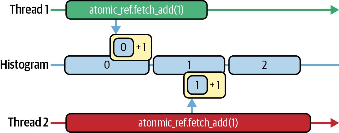
Atomic Counters Atomic counters are the foundation for atomic queues, which allow dynamic work allocation. On modern GPUs, global atomics are serviced and serialized in the on-device L2 cache. This reduces latency versus DRAM round trips when the target line is resident. Atomic counters still incur latency and serialize under contention. But uncontended atomicAdd operations happen extremely quickly by remaining on-chip. An example of two threads incrementing an atomic is shown in Figure 12-1.
Figure 12-1. Superfast, on-chip atomic-memory add operations across multiple threads in the context of a histogram computation
However, atomicAdd does not come for free. It still has latency and, under contention, can serialize threads waiting on the same memory address. As such, the L2 needs to serialize the updates as well. This creates a hotspot, which needs to be optimized. Nsight Compute can help you quantify the cost. In the Memory Workload Analysis section of Nsight Compute, you’ll find atomic_transactions and atomic_transactions_per_request. The atomic transac‐ tions counter represents the total number of L2‐cache atomic transactions, including any replays caused by contention. The atomic transactions per request metric, or con‐ tention ratio, represents the average number of L2 transactions generated by each atomicAdd instruction. When every atomicAdd fires exactly one L2 transaction, your atomic_transac tions_per_request hovers around 1.0, which means it’s paying the bare minimum. If this ratio climbs above 1.0, it signals that the threads are stalling and retrying atomic updates instead of doing useful work. Each retry indicates contention.
Dynamic Scheduling with Atomic Work Queues | 483
The optimization here is to amortize your atomics by grabbing work in batches. So
instead of each thread, or warp, performing an atomicAdd, you batch a group of tasks
per atomic. Here is the before and after with a batch size of 32:
      // Before batching
      int idx = atomicAdd(&queue_head, 1);
      if (idx < N) process(data[idx]);
// After batching const int batchSize = 32; int start = atomicAdd(&queue_head, batchSize); for (int i = start; i < start + batchSize && i < N; ++i) { process(data[i]); } Now a single atomic update awards a warp (or thread block) a whole slice of work— 32 items in this example—before touching the counter again. You still pay one L2 transaction per batch, but you do 32× as much useful work in between. In practice, only one thread per warp performs this atomicAdd to fetch the next batch start index. The thread then broadcasts it to the rest of the warp (e.g., using __shfl_sync). The entire warp then processes those 32 items in parallel. This pro‐ duces one atomic operation per warp instead of per thread, drastically reducing contention. In Nsight Compute you’ll see atomic_transactions plummet and your transactionsper-request collapse back toward 1.0. This proves that you’ve traded costly contention for sustained computation. With modern GPUs in which L2‐cache atomics are exceptionally fast, even a modest batch size of 8 or 16 can eliminate most contention due to the high L2 bandwidth. That said, always verify that you haven’t simply shifted the bottleneck elsewhere. To verify that this optimization hasn’t negatively affected other performance metrics, use Nsight Compute’s Warp Stall Reasons and Register Pressure reports to make sure your fused loop isn’t now limited by register spills or shared‐memory bank conflicts.
                     If atomics are still hot after these optimizations, consider alterna‐
                     tive designs like per-block counters or hierarchical reduction of
                     work distribution.
In short, by batching work per atomic operation, you keep the GPU’s many warps busy doing real computation. This is in contrast to queuing up at a single counter that can’t keep up.
484 | Chapter 12: Dynamic Scheduling, CUDA Graphs, and Device-Initiated Kernel Orchestration
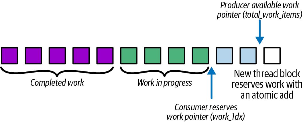
Atomic Queues Let’s now use a global atomic counter to coordinate a dynamic work queue. The goal is to use the atomic counter and atomicAdd to balance arbitrary workloads across all SMs so that no thread, or warp, sits idle. An example of this dynamic work queue is shown in Figure 12-2.
Figure 12-2. Using atomic counter and atomicAdd as a dynamic work queue to balance workloads across SMs and warps
In the next code example (computeKernel), each thread computes a different number of iterations based on idx % 256. Threads with a small value for idx % 256 do very little work, while threads with a large value for idx % 256 will do a lot of work. As a result of this imbalance, threads finish at different times, and some SMs go idle wait‐ ing for the longest threads to complete. Here is the code that uses a static, uneven workload per thread: // uneven_static.cu #include <cuda_runtime.h> #include <cmath>
    __global__ void computeKernel(const float* input, float* output, int N) {
        int idx = blockIdx.x * blockDim.x + threadIdx.x;
        if (idx < N) {
            // Each thread does a variable amount of work based on idx
            int work = idx % 256;
            float result = 0.0f;
            for (int i = 0; i < work; ++i) {
                result += sinf(input[idx]) * cosf(input[idx]);
            }
            output[idx] = result;
        }
    }
    int main() {
        const int N = 1<<20;
float* h_in = nullptr;
Dynamic Scheduling with Atomic Work Queues | 485
            float* h_out = nullptr;
            cudaMallocHost(&h_in, N * sizeof(float));
            cudaMallocHost(&h_out, N * sizeof(float));
for (int i = 0; i < N; ++i) h_in[i] = float(i) / N;
            float *d_in, *d_out;
            cudaMalloc(&d_in, N * sizeof(float));
            cudaMalloc(&d_out, N * sizeof(float));
            cudaMemcpy(d_in, h_in, N * sizeof(float), cudaMemcpyHostToDevice);
            dim3 block(256), grid((N + 255) / 256);
            computeKernel<<<grid, block>>>(d_in, d_out, N);
            cudaDeviceSynchronize();
cudaMemcpy(h_out, d_out, N * sizeof(float), cudaMemcpyDeviceToHost);
            cudaFree(d_in);
            cudaFree(d_out);
            cudaFreeHost(h_in);
            cudaFreeHost(h_out);
            return 0;
      }
                      There isn’t a high-level PyTorch API for dynamic GPU-side work
                      distribution, so we would need to implement it with a custom
                      CUDA kernel. We leave that out for brevity.
In the optimized dynamic task dispatch version shown next, a single global counter (in device memory) is used as a warp-level work queue. We turn the counter into a persistent warp-level work queue using batched atomics. This way, the warps that fin‐ ish early immediately fetch another batch instead of idling: // uneven_dynamic.cu
#include <cuda_runtime.h>
__device__ unsigned int globalIndex = 0;
      // Warp-batched dynamic queue: 1 atomic per active warp
      __global__ void computeKernelDynamicBatch(const float* input,
                                                float* output,
                                                int N) {
        // lane id in [0,31]
        int lane = threadIdx.x & (warpSize - 1);
          while (true) {
            // Elect an active leader each iteration (handles divergence safely)
486 | Chapter 12: Dynamic Scheduling, CUDA Graphs, and Device-Initiated Kernel Orchestration
        unsigned mask = __activemask();
        int leader = __ffs(mask) - 1;
        // Warp leader atomically grabs a contiguous batch for the whole warp
        unsigned int base = 0;
        if (lane == leader) {
          base = atomicAdd(&globalIndex, warpSize);
        }
        // Broadcast starting index to all active lanes in the warp
        base = __shfl_sync(mask, base, leader);
        unsigned int idx = base + lane;
        if (idx >= (unsigned)N) break; // dynamic termination
        // Hoist invariants out of the variable trip-count loop
        // Note: You can also use __sincosf on Blackwell
        float s = sinf(input[idx]);
        float c = cosf(input[idx]);
        int   work = idx % 256;
        float result = 0.0f;
        #pragma unroll 1
        for (int i = 0; i < work; ++i) {
          result += s * c;
        }
        output[idx] = result;
        // loop continues until counter >= N
    }
}
int main() {
    const int N = 1 << 20;
    float *d_in, *d_out;
    cudaMalloc(&d_in, N * sizeof(float));
    cudaMalloc(&d_out, N * sizeof(float));
    // Host buffers (pinned) for a realistic data path
    float *h_in = nullptr, *h_out = nullptr;
    cudaMallocHost(&h_in, N * sizeof(float));
    cudaMallocHost(&h_out, N * sizeof(float));
    for (int i = 0; i < N; ++i) {
        h_in[i] = static_cast<float>(i % 1000);
    }
        // Copy inputs to device
        cudaMemcpy(d_in, h_in, N * sizeof(float),
            cudaMemcpyHostToDevice);
        // Reset global counter
        unsigned int zero = 0;
        // If you call this kernel repeatedly (e.g., in a loop),
        // reset 'globalIndex' to 0 before each launch.
Dynamic Scheduling with Atomic Work Queues | 487
           cudaMemcpyToSymbol(globalIndex, &zero,
               sizeof(unsigned int));
           // Launch with 256 threads per block
           dim3 block(256), grid((N + 255) / 256);
           cudaStream_t stream;
cudaStreamCreateWithFlags(&stream, cudaStreamNonBlocking);
computeKernelDynamicBatch<<<grid, block, 0, stream>>>(d_in, d_out, N);
           cudaStreamSynchronize(stream);
           cudaStreamDestroy(stream);
           cudaDeviceSynchronize();
           // Copy results back and clean up
           cudaMemcpy(h_out, d_out, N * sizeof(float),
                      cudaMemcpyDeviceToHost);
           cudaFree(d_in);
           cudaFree(d_out);
           cudaFreeHost(h_in);
           cudaFreeHost(h_out);
           return 0;
      }
Each warp atomically claims the next batch of tasks of size warpSize (32 threads) from the global queue and processes them in a loop. This makes sure that no SM ever goes idle. This code performs dynamic work distribution implemented with a single global atomic work queue. Here, each warp repeatedly pulls the next batch base index from that global counter. The first thread (if (lane==0)) of each warp, called the warp leader, performs an atomic add to get the starting index of this contiguous block using base=atomic Add(&globalIndex, warpSize). It then broadcasts this base to the rest of its warp using __shfl_sync(__activemask(), base, 0), as described earlier in the chapter. In other words, instead of each thread being tied to a fixed element index, every warp now grabs a contiguous block of tasks from a shared counter. It then computes using idx = base + lane.
488 | Chapter 12: Dynamic Scheduling, CUDA Graphs, and Device-Initiated Kernel Orchestration
All threads in that warp execute the same sin/cos loop for their dynamically fetched indices. As such, work is no longer preassigned per thread. Instead, work is pulled and balanced at runtime using the global atomic queue. Remember that the if (idx >= N) bounds check will cause the warp to exit when there’s no more work to do. This prevents out-of-bounds memory accesses. Other‐ wise, each thread in the warp executes the exact same sin/cos loop as in the static version. In a simple microbenchmark with N = 1 << 20 and work = idx % 256, the statically assigned kernel took about 200 ms, whereas the dynamic-queue version ran in roughly 100 ms. This 2× speedup is a result of eliminating SM idle time and reducing atomic contention. Nsight Compute defines active SM cycles as the fraction of elapsed cycles with at least one active warp. The speedup will vary depending on the work imbalance, but dynamic work distribu‐ tion is an optimization worth exploring any time your profiling shows warp‐idle stalls, low achieved occupancy, or visible timeline gaps from uneven per‐task run‐ times. In these scenarios, especially with moderate imbalance, you can often get a 10%–20% speedup.
               In extreme-imbalance cases, you can get this 2× speedup simply by
               replacing static indexing with an atomic‐driven work queue. For
               mild imbalance, the overhead of the atomic and shuffle may offset
               gains.
In short, dynamic work distribution ensures near-uniform SM utilization since every warp keeps fetching and processing new tasks until the counter exceeds N. This is in contrast to many warps finishing long before the slowest ones and leaving hardware resources unused.
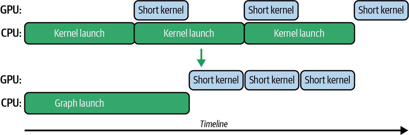
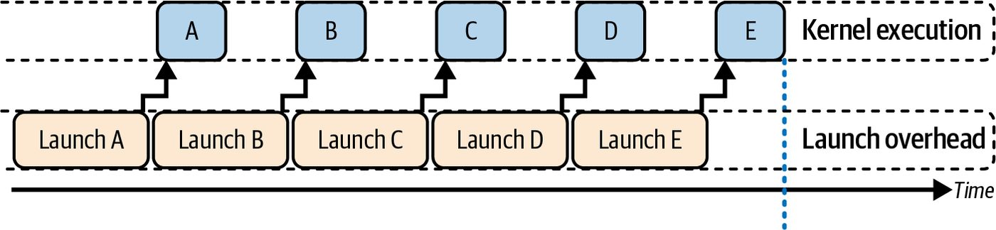
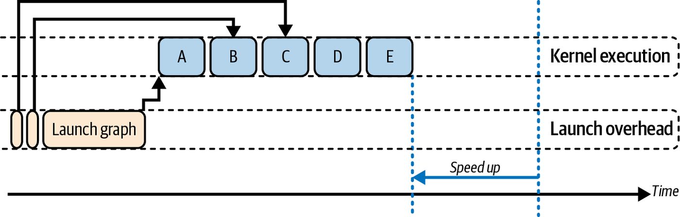
CUDA Graphs When your pipeline consists of multiple kernels, copies, stream-event records, and callbacks, launching them one by one on the host every iteration still incurs CPU overhead. CUDA Graphs let you capture that entire workflow once and replay it repeatedly with essentially zero CPU overhead. Figure 12-3 compares kernel launches without (top) and with (bottom) CUDA Graphs.
CUDA Graphs | 489
Figure 12-3. Kernel-launch timeline without (top) and with (bottom) CUDA Graphs
Why use CUDA Graphs? First, they cut down launch overhead. Multiple small ker‐ nels or copies can be launched with essentially one CPU call. Second, they enable bet‐ ter scheduling on the GPU. The work is submitted as a batch, so the CUDA driver can potentially reduce some internal latency between operations. Also, with CUDA Graphs, dependencies are known upfront, so there’s less need for the CPU to synchronize in between. In the context of memory transfers, a CUDA Graph ensures that asynchronous copies and kernel executions are linked as depen‐ dencies correctly without any manual synchronization. It doesn’t inherently overlap copies and kernels more so than normal streams would, but a CUDA Graph stream‐ lines their execution.
PyTorch, Inference Engines, and CUDA Graphs AI frameworks like PyTorch leverage CUDA Graphs under the hood for static por‐ tions of deep learning models. Specifically, PyTorch supports a torch.cuda.Graph context for capturing a sequence of operations. In addition, PyTorch continues to optimize its internals to use CUDA Graphs for predictable portions of code. High-performance inference engines like vLLM and NVIDIA’s TensorRT-LLM can also leverage CUDA Graphs by capturing a model’s execution into a set of predefined graphs for different sequence-length ranges and input-batch sizes. When graph cap‐ ture is enabled, these systems often bucket or pad inputs to match supported graph batch sizes so that captured graphs can be replayed with fixed shapes. This can signif‐ icantly reduce latency for large-scale, production inference workloads.
490 | Chapter 12: Dynamic Scheduling, CUDA Graphs, and Device-Initiated Kernel Orchestration
For example, you would capture one CUDA Graph per batch size during startup or model‐load time. Then, at runtime, you would launch the precaptured graph that matches the incoming request’s batch size.
              PyTorch compiler mode='reduce-overhead' may wrap eligible seg‐
              ments in CUDA Graphs to reduce launch overhead, subject to cap‐
              ture requirements such as static tensor addresses and CUDA-only
              regions. It does not guarantee graphing of all code paths. And it
              may increase memory use due to pooled buffers. Always profile to
              confirm benefits on your model.
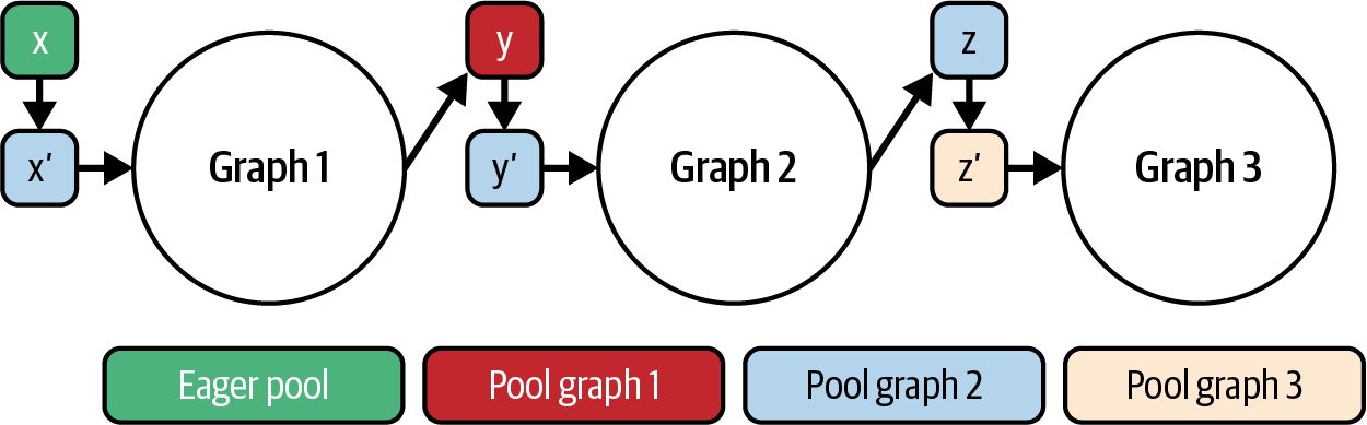
Memory Pools for CUDA Graphs One important consideration is memory management with CUDA Graphs. Memory operations inside a CUDA Graph obey the same rules as in CUDA streams. If you allocate GPU memory inside the capture, that allocation becomes part of the graph execution. You generally want to avoid allocating GPU memory inside your graph and preallo‐ cating memory outside of the graph. Many frameworks, such as PyTorch, use static memory pools with CUDA Graphs, as shown in Figure 12-4. The use of static mem‐ ory pools keeps memory allocations from becoming part of the captured graph sequence.
Figure 12-4. PyTorch uses static memory pools for CUDA Graphs
While CUDA Graphs won’t make an individual memory copy or kernel execution faster, they can automatically overlap independent data transfers and computations within the graph—similar to CUDA streams. This eliminates the per-iteration CPU scheduling and is made possible since the dependency graph is known upfront.
CUDA Graphs | 491
Capturing a CUDA Graph with a CUDA Stream To capture a graph, you call cudaStreamBeginCapture() on a stream, enqueue all your memory transfers (cudaMemcpyAsync()), kernel launches, events (cudaEvent Record()), and callbacks (cudaLaunchHostFunc()), then call cudaStreamEndCap ture() to create a CUDA Graph definition (cudaGraph_t). The CUDA driver can then launch the CUDA Graph with cudaGraphLaunch() every iteration. Because the CUDA driver knows the entire dependency graph in advance, it replays the prebuilt stream sequence directly on the GPU. This incurs minimal launch overhead.
                     cudaGraphExecUpdate, discussed in the next section, allows limited
                     changes to a captured graph for scenarios where sizes, dimensions,
                     or pointers change between iterations. This is useful if the size of
                     the inputs varies since you can just update the graph’s node param‐
                     eters instead of recapturing a whole new graph for each new input
                     size.
Even if only some of your pipeline is repetitive, CUDA Graphs can capture that por‐ tion. For example, if you always perform a Host → Device copy, followed by two ker‐ nels, followed by a Device → Host copy, you can capture just that subgraph and replay it with a single function call. To replay the CUDA Graph, you supply the stream handles, and the GPU executes the sequence of operations without additional CPU instructions. This ties directly to inter-kernel concurrency because CUDA Graphs let you maintain complex overlap‐ ping behavior by mixing asynchronous copies, fine-grained event barriers, and ker‐ nels—while removing the CPU as a bottleneck entirely. Typically, you do a replay dry run to ensure correctness. You would instantiate the graph by creating a cudaGraphExec_t executable graph and then launch it with a sin‐ gle graph-replay invocation. When you launch the captured graph, the runtime will execute all the operations in the correct order on the GPU. To show the usage of CUDA Graphs, consider a simple sequence of kernels. Here we show a code snippet for capturing and launching a CUDA Graph in both C++ and PyTorch: cudaStream_t stream; cudaStreamCreateWithFlags(&stream, cudaStreamNonBlocking); cudaGraph_t graph; cudaGraphExec_t instance;
cudaStreamBeginCapture(stream, cudaStreamCaptureModeGlobal);
// Enqueue operations on 'stream' as usual
492 | Chapter 12: Dynamic Scheduling, CUDA Graphs, and Device-Initiated Kernel Orchestration
    kernelA<<<grid, block, 0, stream>>>(d_X);
    kernelB<<<grid, block, 0, stream>>>(d_Y);
    kernelC<<<grid, block, 0, stream>>>(d_Z);
    cudaStreamEndCapture(stream, &graph);
    cudaGraphInstantiate(&instance, graph, nullptr, nullptr, 0);
    // Now 'instance' can be launched in a loop
    for (int iter = 0; iter < 100; ++iter) {
        cudaGraphLaunch(instance, stream);
        // No per-kernel sync needed; graph ensures dependencies
    }
    cudaStreamSynchronize(stream);
// (Destroy graph and instance when done) cudaGraphExecDestroy(instance); cudaGraphDestroy(graph); In this pseudocode, we begin capturing on a CUDA stream, launch three kernels (A, B, and C) in sequence on that stream, and end capture to obtain a graph. Then we instantiate the graph. Now we can replay the entire sequence A → B → C by calling cudaGraph Launch (instance, stream) as many times as we want. We only pay for the cost of a single launch per iteration instead of three separate launches. And the GPU executes kernels A, B, and C in the same sequence they were recorded, or back-to-back in this case. We will synchronize after the loop to ensure that all iterations are complete. As mentioned earlier, high-level AI frameworks like PyTorch support CUDA Graphs. PyTorch provides Python developers with near-native CUDA performance without requiring deep knowledge of CUDA C++. Here, we show PyTorch’s torch.cuda.Graph context manager to capture and replay operations: import torch, time
X = torch.randn(1<<20, device='cuda')
    # Define operations for reference
    def opA(x): return x * 1.1
    def opB(x): return x + 2.0
    def opC(x): return x.sqrt()
    # Persistent buffers for pointer stability
    static_x = torch.empty_like(X)
    static_y = torch.empty_like(X)
    static_z = torch.empty_like(X)
    static_w = torch.empty_like(X)
    # Warm up once to initialize CUDA kernels and caches
    _ = opC(opB(opA(X)))
    torch.cuda.synchronize()
CUDA Graphs | 493
      # Seed the static input before capture
      static_x.copy_(X)
      # Capture the graph
      g = torch.cuda.CUDAGraph()
      stream = torch.cuda.Stream()
      torch.cuda.synchronize()
      with torch.cuda.graph(g, stream=stream):
          # Record A then B then C using out parameters to avoid allocations
          torch.mul(static_x, 1.1, out=static_y)
          torch.add(static_y, 2.0, out=static_z)
          torch.sqrt(static_z, out=static_w)
# Replay the captured graph 100 times for i in range(100): # If inputs change, copy new values into static_x before replay # static_x.copy_(new_X) g.replay() In production you should allocate persistent input and output buffers so captured kernels see fixed memory addresses. For example, create static_y = torch.empty_like(X) before capture, and then inside the graph write static_y.copy_(opA(X)). This avoids allocations during capture and satisfies the stability rules of CUDA Graph pointers. PyTorch CUDA Graphs requires that replay uses the same memory addresses for captured tensors. In this PyTorch example, we define operations opA, opB, and opC. In practice, these could be neural network layers or any GPU operation. We run one warm-up pass opC(opB(opA(X))) to ensure that all kernels, memory allocations, and library con‐ texts (e.g., cuBLAS/cuDNN) are initialized upfront. This is needed because a CUDA Graphs capture won’t record these lazy setup steps.
                     Skipping the warm-up pass may cause your graph capture to fail or
                     introduce unexpected stalls when lazy initializations occur.
We first warm up the GPU by running the sequence once to initialize all kernels and libraries. Then we capture the forward (A), transform (B), and backward (C) opera‐ tions into a single torch.cuda.CUDAGraph by enclosing them in the with torch.cuda.graph(g, stream=stream): Python context manager block on a fresh CUDA stream. After capture, calling g.replay() 100 times launches the entire A → B → C pipeline with one host call per iteration. The results are summarized in Table 12-1.
494 | Chapter 12: Dynamic Scheduling, CUDA Graphs, and Device-Initiated Kernel Orchestration
Table 12-1. Impact of CUDA Graphs on iteration overheads Metric Before CUDA Graphs After CUDA Graphs CPU launch calls per 100 iterations 300 separate kernel launches 100 graph replays (1 per iteration) Host synchronization calls 300 cudaDeviceSynchronize calls 0 Average GPU idle between kernels ~3 µs gaps per iteration 0 µs (continuous back-to-back execution) End-to-end iteration latency ~1.00 ms ~0.75 ms (25% faster)
                      Note: The numeric values in all metrics tables are illustrative to
                      explain the concepts. For actual benchmark results on different
                      GPU architectures, see the GitHub repository.
Here we see that CUDA Graphs eliminate per-iteration CPU scheduling and hostdevice handshakes. This is because the GPU work for each iteration is batched into a single g.replay() call instead of three separate kernel launches. As a result, iterations execute 25% faster since the CPU simply issues lightweight replay commands and stays fully asynchronous to the GPU. There are some common pitfalls when using CUDA Graphs, and it’s important to handle them appropriately. For example, if your workload size changes, a captured graph might not be valid. This would require a recapture or a call to cudaGraphExec Update, which we cover in the next section. Certain CUDA API calls—like allocating memory and host-device synchronization primitives—should generally not be included in a graph capture. While modern ver‐ sions of CUDA Graphs support limited memory management operations inside a captured graph, it’s recommended to perform all memory allocations before the cap‐ ture. You must also ensure that the data used in the graph remains at the same mem‐ ory addresses.
                      The requirement for memory to remain at the same memory
                      address during graph execution is a primary reason why frame‐
                      works like PyTorch use static memory pools with CUDA Graphs.
                      For example, PyTorch provides the torch.cuda.graph_pool_han
                      dle() API to create a dedicated memory pool for pointer-stable
                      CUDA graph capture. Using a separate allocator pool ensures that
                      tensor addresses remain fixed across captures and replays. This sat‐
                      isfies the pointer stability requirement. Between iterations, update
                      inputs by copying into static tensors. Don’t reallocate the tensors
                      on every iteration.
CUDA Graphs | 495
You should also avoid including any host‐side callbacks or unsupported operations inside a CUDA Graphs capture. This includes things like print(), random number generator (RNG) calls, nested captures, and new memory allocations. This is because the graph must record a pure, deterministic sequence of GPU work. In addition, all tensors used in the capture must already be allocated at fixed addresses with fixed shapes. Resizing or calling cudaMalloc during capture will break the graph.
Dynamic Graph Update Once you’ve recorded a CUDA Graph, you don’t need to throw it away just because some launch parameters change. Instead of recapturing, you call the graph-update API to update grid/block dimensions, pointer addresses, or kernel parameters directly in the existing graph. The graph-update API includes cudaGraphExecUpdate and the lower-level cudaGraphExecKernelNodeSetParams. cudaGraphExecUpdate lets you swap a kernel node with a new one of the same shape. For example, you can swap in a different fused kernel implementation—as long as it’s the same shape. The CUDA runtime will validate your tweaks and let you replay the modified graph immediately. This avoids the cost of a full capture.
                     As of this writing, you cannot add or remove nodes arbitrarily. The
                     runtime will return an error if an update violates what the existing
                     graph can handle. In this case, you must capture a new graph.
For example, consider our three-kernel A → B → C graph from earlier, using your maximum batch size. During each inference loop, you simply update Kernel B’s launch dimensions to match the current batch, then replay the same graph. This reduces overhead for semistatic workloads in which the overall pipeline is fixed but a few parameters may vary. In practice, a typical workflow is three steps. First, capture a template graph using the maximum expected sizes (e.g., the largest batch). For example, you might capture your graph with a maximum batch size of 128. Later, if a request comes in with batch 64, you call cudaGraphExecUpdate to adjust the launch parameters to 64—and per‐ haps update the memory pointers to a smaller buffer. Using cudaGraphExecUpdate keeps you from having to rebuild the graph when kernel parameters, grid/block dimensions, or memory addresses change. And it takes only a few microseconds, so you preserve the fast sub-100 µs launch overhead of a CUDA Graph replay. In addition, you maintain the flexibility of adjusting key parameters at
496 | Chapter 12: Dynamic Scheduling, CUDA Graphs, and Device-Initiated Kernel Orchestration
runtime. Note that incompatible changes will return an error status and require recapture. If you do need to change the graph’s structure to specify a different number of kernels, for instance, you can fall back to a recapture-then-update workflow. In this case, you wrap one iteration of your code with cudaStreamBeginCapture and cudaStreamEndCapture to build the new graph. Then use the lighter-weight cudaGraphExecUpdate for minor tweaks on subsequent runs. In effect, dynamic graph updates let you create “parameterized” or conditional execu‐ tion paths entirely on the GPU. Whenever you have a high-frequency loop of GPU work but only a few changing parameters, like batch size, you can capture once, update quickly, and enjoy both minimal CPU overhead and the adaptability that your use case requires.
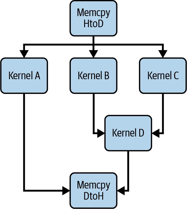
Device-Initiated CUDA Graph Launch Now that you understand how to launch and adapt a captured pipeline from the CPU with low overhead, the next step is to remove the CPU from the launch decision entirely. With device-initiated CUDA Graph launches, a running GPU kernel can trigger a prerecorded graph directly on the device and avoid the host entirely. To enable device-side launch, first capture the graph as usual on the host. Then instantiate it with cudaGraphInstantiate and pass cudaGraphInstantiateFlag DeviceLaunch. After instantiation, upload the executable with cudaGraphUpload on a host stream before any device-side launch. You then upload the graph to GPU memory using cudaGraphUpload. This must be done before the GPU can launch the graph. (Attempting a device launch without uploading the graph will cause an error.) In practice, this embeds a “graph launch” node, or calls the device‐side graph API, inside your persistent or dynamic kernel. When the time comes, the GPU will kick off the entire graph on a stream that it owns, as shown in Figure 12-5. Device-initiated graph launches keep data-driven workflows completely on the GPU. Your kernel is responsible for computing the decision conditions, not the CPU. As such, it can spawn the next graph directly, eliminate CPU round trips, and further reduce latency. Because the graph is already resident on the GPU and no CPU-GPU handshake is needed, device-initiated launches remove host scheduling from the critical path and can reduce end-to-end latency in host-bound loops. In practice, device-initiated CUDA graph launches have shown roughly 2× lower launch latency compared to equivalent host-side graph launches. And the overhead stays flat even as the graph grows in size or complexity.
CUDA Graphs | 497
Figure 12-5. Sequence of operations (nodes for kernels and data transfers) and their dependencies (edges) launched by a CUDA Graph
Device-launch graph latency is not impacted by how many nodes or parallel branches are in the graph. This is in contrast to host-launch graph latency, which would increase with a larger graph due to CPU scheduling overhead. In addition, device launches scale well with graph width. As more parallel nodes are added, host-side launching would suffer from additional synchronization costs, but the device launch latency remains nearly flat. Debugging device-launched graphs can be tricky, but tools like Nsight Systems will show the child graphs on the GPU timeline as separate streams of work. It’s recom‐ mended to use NVTX markers in the parent kernel before and after cuda Graph Launch calls to mark where device launches occur. This can help verify that the graphs run as expected in relation to the parent thread. Inside your device code, you launch the graph with the simple API, cuda Graph Launch(graphExec, stream). The runtime uses special, reserved cudaStream_t val‐ ues to distinguish between the following supported launch modes: “fire-and-forget” (cudaStreamGraphFireAndForget), “tail” (cudaStreamGraphTailLaunch), and “sib‐ ling” (cudaStreamGraphFireAndForgetAsSibling). These modes will automatically enforce the correct ordering in the CUDA stream without any host intervention. In a fire-and-forget launch, the child graph begins executing immediately and con‐ currently with the launching parent kernel. The parent kernel doesn’t wait for the child to finish—much like launching an independent thread of work. Fire-and-forget launches are useful for spawning asynchronous tasks from within a kernel.
498 | Chapter 12: Dynamic Scheduling, CUDA Graphs, and Device-Initiated Kernel Orchestration
                A graph can have up to 120 total fire-and-forget graphs during the
                course of its execution.
By contrast, a device-initiated graph tail launch defers execution of the graph until the launching kernel reaches a synchronization point or completes. This effectively queues the graph to run after the current kernel as a continuation, as shown in Figure 12-6.
Figure 12-6. Tail launches enqueued by a given graph will execute one at a time, in order of when they were enqueued
Tail launches are especially powerful when implementing GPU-resident work sched‐ ulers. A persistent “scheduler” kernel can tail-launch a graph, then relaunch itself once that graph finishes. This technique effectively creates a loop on the GPU without requiring host re-invocation. To relaunch itself, the kernel calls cudaGetCurrent GraphExec() to get a handle to its own executing graph. It then launches the graph using cudaGraphLaunch(..., cudaStreamGraphTailLaunch) to enqueue itself again. Additionally, tail graphs can perform additional tail launches. In this case, the new tail launches will execute before the previous graph’s tail launch, as shown in Figure 12-7.
Figure 12-7. Tail launches enqueued from multiple graphs
                You can have up to 255 pending tail launches enqueued in a CUDA
                Graph. However, when it comes to a self-tail-launch (e.g., a graph
                enqueues itself for relaunch), you can have only one pending self-
                tail-launch at a time.
CUDA Graphs | 499


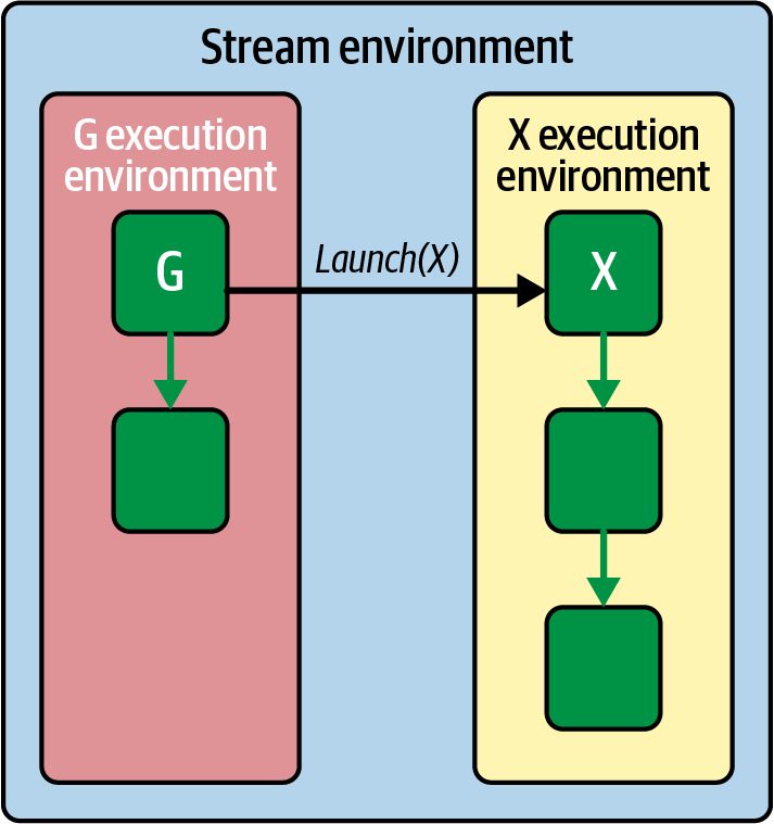
A sibling launch is a variation of fire-and-forget in which the launched graph exe‐ cutes as a peer to the parent graph—instead of as a child. Additionally, the sibling runs in the parent’s stream environment. This means it runs immediately and inde‐ pendently but without delaying any tail launches of the parent graph, as shown in Figure 12-8.
Figure 12-8. Sibling graph launch in the parent’s stream environment
For this mode, you can use cudaGraphLaunch(graphExec, cudaStreamGraphFireAnd ForgetAsSibling) to launch in “sibling mode.” This submits the graph as a sibling of the current graph’s execution environment. When using device-initiated CUDA Graphs, you need to carefully manage dependen‐ cies. For instance, if the launched kernel must consume results from the graph, a tail launch is appropriate because the parent kernel will pause until the graph’s work is done. In contrast, if the launched graph is more of a side task, the fire-and-forget mode allows the parent kernel to proceed without waiting. In practice, device-initiated CUDA Graphs open up new patterns. For example, imag‐ ine a GPU compression pipeline where a kernel must choose between different com‐ pression algorithms based on data content. Rather than ending the kernel and telling the CPU to launch the chosen compression kernel, the GPU kernel can directly launch a prerecorded graph corresponding to, say, “LZ compression” or “Huffman compression.”
500 | Chapter 12: Dynamic Scheduling, CUDA Graphs, and Device-Initiated Kernel Orchestration
In this compression example, the GPU never idles waiting for the CPU to decide. Let’s take a look at another useful pattern that combines atomic queues/counters and device-initiated, tail-launched CUDA Graphs for LLM inference scheduling inside of a persistent kernel.
Atomic Queues and Device-Initiated CUDA Graphs for In-Kernel Persistent Scheduling We can combine our atomic‐counter work queue from earlier with device‐initiated graph tail launches. Consider an LLM inference loop use case, which uses a CUDA Graph to perform a decode by capturing a graph that includes the transformer‐block’s forward pass (attention + feed-forward). A lightweight, persistent scheduler kernel can use atomicAdd(&queueHead,1) to claim the next work item. It then tail‐launches the precaptured decode CUDA Graph to compute the output and immediately loops back for the next item in the queue. When each CUDA Graph completes, the in-kernel scheduler loop grabs the next index using atomicAdd(&queueHead,1) and tail‐launches another decode graph. This effectively creates a fully GPU‐resident scheduler that both decides and executes tasks without touching the CPU. By chaining these tail launches, each token is processed start-to-finish on the device with virtually zero CPU overhead. And since the CPU never reenters the critical path, SMs remain fully utilized, per-token latency drops, and you can adapt to different sequence lengths and batch sizes on the fly. To do this, you simply update graph parameters or switch between prerecorded graphs.
Conditional Graph Nodes In a traditional CUDA Graph, every node and its dependencies are fixed at capture time, forcing any decision-making logic back to the host. Conditional graph nodes break this rigidity by deferring branch decisions to the GPU itself—based on a small “condition handle” associated with the node. As the graph executes, the GPU evaluates that handle and selectively runs one of its body subgraphs (or loops through it) without ever returning control to the CPU. Specifically, conditional graph nodes let you embed the control flow (IF, IF/ELSE, WHILE, SWITCH) directly into CUDA Graphs to run on the GPU device. Condi‐ tional graph nodes eliminate host round trips and can provide significant perfor‐ mance gains on modern GPUs.
CUDA Graphs | 501
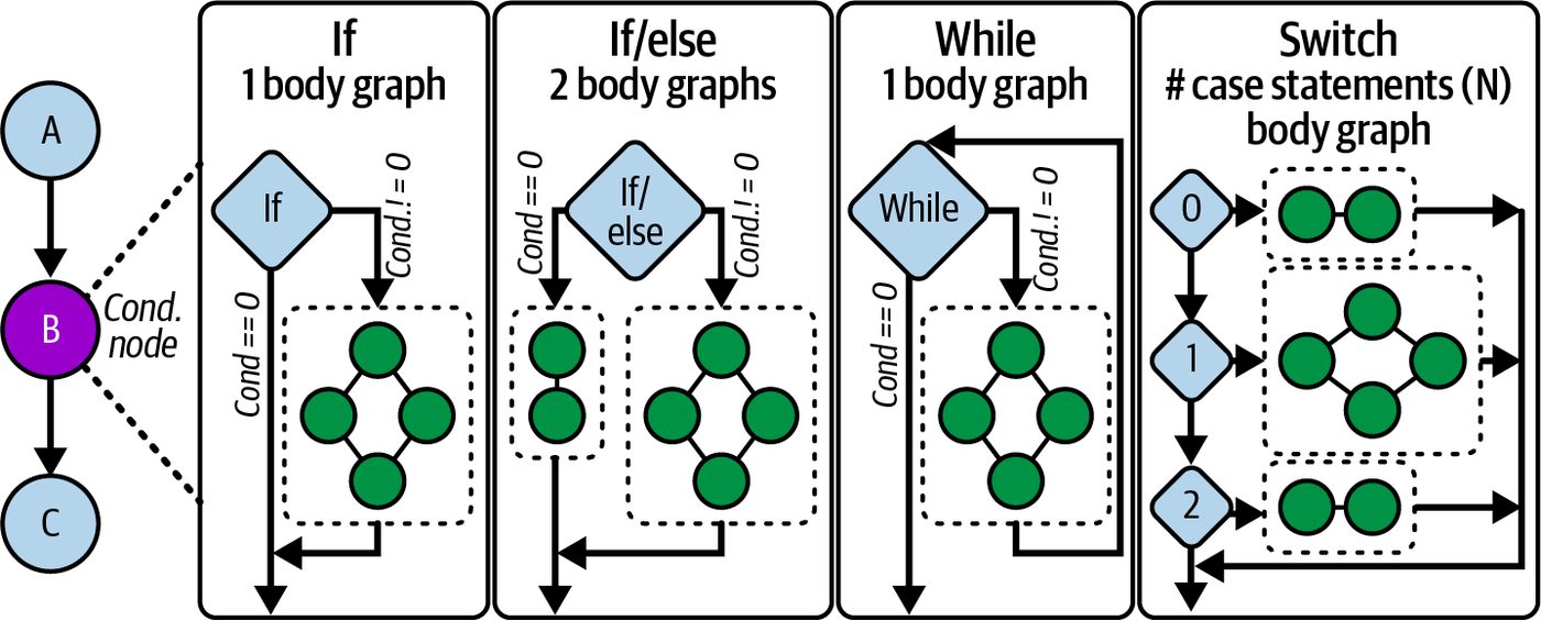
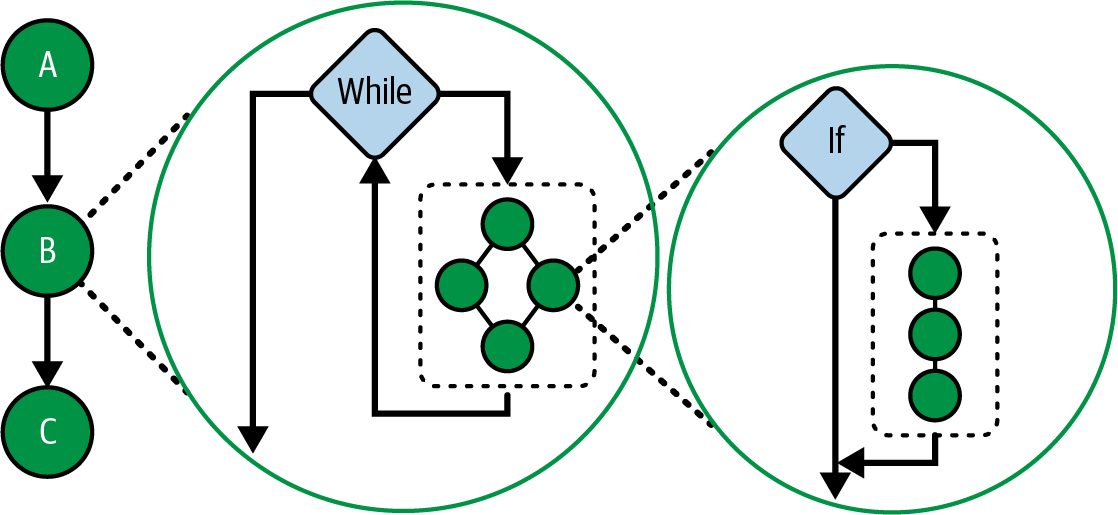
In essence, conditional graph nodes let you control graph execution based on values computed in device kernels—all without involving the CPU. This capability allows complex branching workflows to be implemented as a single, repeatable graph launch. CUDA Graphs support multiple types of conditional nodes, as shown in Figure 12-9: IF Executes its single-body graph exactly once when the condition is nonzero. IF/ELSE By specifying two body graphs, one is chosen when the condition is true, the other when false. WHILE Repeatedly executes its body graph as long as the condition remains nonzero, checking again after each iteration. SWITCH Holds N body graphs and executes the ith one when the condition equals i; if the condition ≥ N, it skips execution altogether.
Figure 12-9. Types of conditional graph nodes
Next is an example showing how to create and populate an IF conditional node. Note the use of cudaGraphSetConditional to write the flag that controls the IF node. In this case, the condition checks if the sum is greater than a given threshold. This way, if the data meets the given criteria (flag = 1u), it runs the next subgraph. Otherwise, if the condition is not met, the conditional node does not run the subgraph: #include <cuda_runtime.h> #include <cstdio>
      // Device kernel that computes and sets the condition handle
      __global__ void setHandle(cudaGraphConditionalHandle handle,
                                int *data, size_t N) {
502 | Chapter 12: Dynamic Scheduling, CUDA Graphs, and Device-Initiated Kernel Orchestration
    // Example threshold
    constexpr int threshold   = 123456;
    // Test whether the sum of data exceeds a threshold
    //     using a custom reduce_sum() function
    //     (recommended to implement this with
    //     CUB's DeviceReduce::Sum routine.)
    unsigned int flag =
        (reduce_sum(data, N) > threshold) ? 1u : 0u;
    cudaGraphSetConditional(handle, flag);
}
// A simple body kernel that runs only if flag != 0 __global__ void bodyKernel() { printf("Conditional body executed on GPU!\n"); }
int main() {
    cudaStream_t stream;
    cudaStreamCreateWithFlags(&stream,
        cudaStreamNonBlocking);
    // 1) Create the graph
    cudaGraph_t graph;
    cudaGraphCreate(&graph, 0);
    // 2) Create a condition handle associated with graph
    cudaGraphConditionalHandle condHandle;
    cudaGraphConditionalHandleCreate(&condHandle, graph);
    // 3) Add the upstream kernel node to set the handle
    cudaGraphNode_t setNode;
    cudaKernelNodeParams setParams = {};
    setParams.func           = (void*)setHandle;
    setParams.gridDim        = dim3(1);
    setParams.blockDim       = dim3(32);
    // 4) Allocate input data
    constexpr size_t N              = 1 << 20;
    int*             d_data         = nullptr;
    cudaMalloc(&d_data, N * sizeof(int));
    void* setArgs[] = { &condHandle, &d_data, &N };
    setParams.kernelParams = setArgs;
    cudaGraphAddKernelNode(&setNode, graph, nullptr, 0,
        &setParams);
    // 5) Add the IF conditional node
    cudaGraphNode_t condNode;
    cudaConditionalNodeParams ifParams = {};
    ifParams.handle = condHandle;
CUDA Graphs | 503
           ifParams.type   = cudaGraphCondTypeIf;
           // One-node body graph, in this case
           ifParams.size   = 1;
           cudaGraphAddConditionalNode(&condNode,
                                       graph,
                                       &setNode,
                                       1,
                                       &ifParams);
           // 6) Populate the body graph: one kernel that prints a message
           cudaGraph_t bodyGraph = ifParams.phGraphOut[0];
           cudaGraphNode_t bodyNode;
           cudaKernelNodeParams bodyParams = {};
           bodyParams.func         = (void*)bodyKernel;
           bodyParams.gridDim      = dim3(1);
           bodyParams.blockDim     = dim3(32);
           cudaGraphAddKernelNode(&bodyNode, bodyGraph, nullptr,
               0, &bodyParams);
           // 7) Instantiate, upload, and launch the graph on the device
           cudaGraphExec_t graphExec;
           cudaGraphInstantiate(&graphExec, graph, nullptr, nullptr,
           cudaGraphInstantiateFlagDeviceLaunch);
           cudaGraphUpload(graphExec, stream);
           cudaGraphLaunch(graphExec, stream);
           // 8) Wait for completion and clean up
           cudaStreamSynchronize(stream);
           cudaGraphExecDestroy(graphExec);
           cudaGraphDestroy(graph);
           cudaStreamDestroy(stream);
cudaFree(d_data);
           return 0;
      }
Here, we create a new CUDA Graph with cudaGraphCreate, which will hold all sub‐ sequent nodes. We then create a condition handle using cudaGraphConditional HandleCreate. (This associates a small integer value to the graph that can be set on the device.) An upstream kernel, setHandle, is then added. This kernel runs on one thread to avoid race conditions. It then calls cudaGraphSetConditional to write the flag that controls the IF node. The IF conditional node is added with cudaGraphAddConditionalNode—specifying cudaGraphCondTypeIf and size=1. This defines how many conditional branches or iterations we plan to support.
504 | Chapter 12: Dynamic Scheduling, CUDA Graphs, and Device-Initiated Kernel Orchestration
Here, we allocate one empty subgraph (body) to be executed if the conditional flag returns nonzero. The body graph is retrieved from ifParams.phGraphOut[0] and populates it by adding bodyKernel, which simply prints a message when executed. After graph construction, call cudaGraphInstantiate to produce an executable graph object. To launch a graph from device code, you must instantiate it with the cudaGraphInstantiateFlagDeviceLaunch flag and upload it with cudaGraphUpload before any device-side launch. Launching with cudaGraphLaunch on a CUDA stream triggers execution of the upstream set-handle kernel, the conditional check, and then, if the flag was set, the body kernel. And all of this happens directly on the GPU, as shown in Figure 12-10.
Figure 12-10. Additional processing (body subgraph) if condition is met
We then synchronize the stream with cudaStreamSynchronize to wait for comple‐ tion. Finally, we clean up by destroying the instantiated graph, the graph itself, and the stream. To minimize race conditions, it’s important to always set the condition in a single thread (e.g., if (threadIdx.x == 0)). And make sure that the preceding kernels flush memory to make the value visible before the conditional node executes. Conditional nodes can be nested as well. For instance, a WHILE node’s body can con‐ tain an IF node, as shown in Figure 12-11. This allows multilevel decision logic without requiring CPU hops.
CUDA Graphs | 505
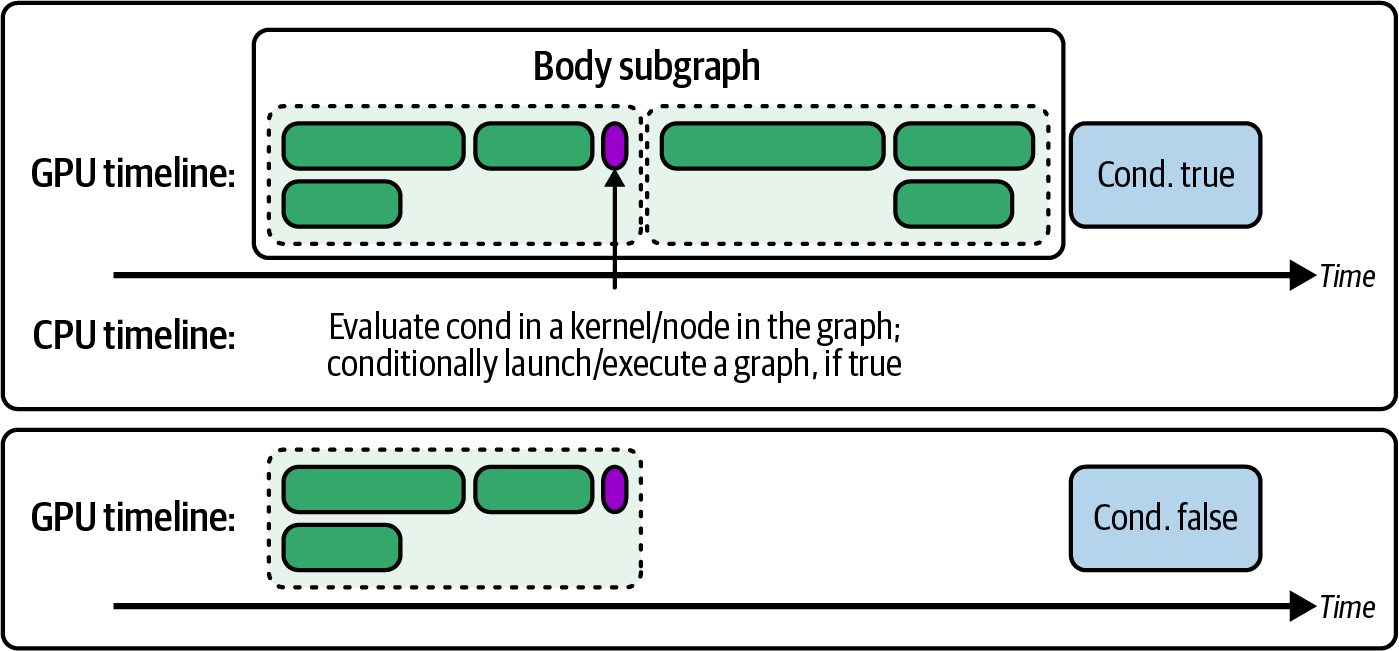
Figure 12-11. Nested conditional graph nodes
In short, you should use conditional graph nodes to keep decisions on the GPU, reduce CPU overhead, and express complex control flow directly in your CUDA Graph. Because graph creation costs can be amortized over many iterations, repre‐ senting dynamic workflows entirely on-device can produce significant performance improvements.
                    As of this writing, PyTorch’s CUDA Graphs API does not provide a
                    way to create conditional CUDA graph nodes directly with the
                    Python. Support for conditional graph execution in frameworks
                    and tools is evolving. As of this writing, this feature requires cus‐
                    tom C++ integrations if you need to implement if/while/switch
                    nodes with PyTorch.
Dynamic Parallelism Previously, we saw how the device‐initiated CUDA Graph launches capture and replay fixed sequences of operations with minimal CPU involvement. But that model expects that your entire execution flow is known ahead of time, which isn’t always possible. Many workloads change shape at runtime based on input data, intermediate results, or problem complexity. That’s where Dynamic parallelism (DP) comes in. DP gives your GPU kernels the power to spawn new work for themselves instead of waiting on the CPU. Whereas CUDA Graphs require you to know your entire pipe‐ line in advance, DP lets a running “parent” kernel examine its own outputs and decide on the fly how many “child” kernels to launch next. This is a game-changer for truly irregular problems—hierarchical reductions, adaptive mesh refinement, and graph traversals—where the number of subsequent tasks becomes clear only as you process your data. Imagine an inference pipeline that occasionally needs a special “plugin” model evalu‐ ation for certain inputs. In a CPU-driven flow, you’d run Kernel A, copy its results
506 | Chapter 12: Dynamic Scheduling, CUDA Graphs, and Device-Initiated Kernel Orchestration
back to the host, decide whether to launch Kernel B, and then issue that launch— leaving the GPU idle during the round trip. With DP, Kernel A inspects its outputs and, if the condition holds, launches Kernel B directly on the device. The entire decision-and-dispatch happens inside one GPU-resident workload, collapsing the idle gap and keeping SMs busy. In the context of an LLM, most tokens follow the standard transformer path, but some require an auxiliary attention block. A DP-enabled transformer kernel can detect those special tokens at runtime and tail-launch the extra attention kernel only for those positions—no host intervention, no wasted cycles. NVIDIA’s libraries already exploit DP for similar patterns in adaptive algorithms: new subtasks emerge dynamically as data flows through the computation. You’ll know DP is right for you when your profiler timeline shows a back-to-back pattern like Kernel A → GPU idle gap → Kernel B. Here, the idle time corresponds to the CPU preparing the next launch. Replacing that gap with a device-side launch keeps every SM occupied and slashes the latency between dependent stages. Of course, the performance benefits of DP don’t come for free. Each child launch uses GPU scheduling resources and requires additional stack space. To avoid “stack over‐ flow” errors, you may need to bump the runtime stack size with cudaDeviceSet Limit(cudaLimitStackSize, newSize). CUDA will warn you if you hit its default limit. On a related note, CUDA has a maximum limit on how many child-kernel launches can be pending. By default, CUDA allows 2,048 outstanding device launches at one time. However, this is configurable. If a parent kernel needs to spawn more than 2,048 child kernels because it’s using a large loop to launch thousands of tiny kernels, you can raise this limit using the API cudaDeviceSetLimit(cudaLimitDevRuntimePendingLaunchCount, newLimit). Other‐ wise, exceeding the default 2,048 limit will cause a runtime error. In practice, the default value is usually enough for most uses. But it’s an important consideration for extreme cases.
               When spawning many child kernels on the GPU, be sure to moni‐
               tor device memory usage since each pending child-kernel launch
               reserves resources and may exceed the hard limits of your GPU
               hardware.
Because DP adds some instruction-level overhead, it’s best reserved for cases where static orchestration like persistent kernels, streams, or CUDA Graphs would other‐ wise leave the GPU idling while the CPU decides the next step. In other words, when
Dynamic Parallelism | 507
your workload is truly a fixed sequence of operations, you’re often better off captur‐ ing it as a CUDA Graph and replaying it device-side. When your work emerges dynamically from the data itself, DP lets you keep both scheduling and execution entirely on the GPU. This will deliver better scaling and lower end-to-end latency for nested, data-dependent, or unpredictable parallelism.
                     Because DP incurs per-launch overhead and consumes pending-
                     launch slots, use DP when new parallelism emerges from the data
                     at runtime and can’t be expressed as a pre-recorded CUDA Graph.
                     In contrast, favor device-launched CUDA Graphs when the control
                     flow is expression-level and repeated since CUDA Graphs amortize
                     the costs.
Let’s compare two implementations of a simple parent-child workflow. The host-
driven version shown next launches a parent kernel, waits for it to finish, then issues
two child kernels from the CPU. This leaves the GPU idle during those decision gaps:
      // dp_host_launched.cu
      #include <cuda_runtime.h>
      __global__ void childKernel(float* data, int N) {
          int idx = blockIdx.x * blockDim.x + threadIdx.x;
          if (idx < N) {
              data[idx] = data[idx] * data[idx];
          }
      }
      __global__ void parentKernel(float* data, int N) {
          // Parent does setup work. Here, CPU decides on child launches.
          if (threadIdx.x == 0 && blockIdx.x == 0) {
              // maybe mark regions or compute flags here
          }
      }
      int main() {
          const int N = 1 << 20;
          float* d_data;
          cudaMalloc(&d_data, N * sizeof(float));
          // ... initialize d_data ...
           // 1) Launch parent and wait
           cudaStream_t s; cudaStreamCreateWithFlags(&s, cudaStreamNonBlocking);
parentKernel<<<1,1,0,s>>>(d_data, N);
cudaStreamSynchronize(s);
           // 2) CPU splits work in half and launches children
           int half = N / 2;
508 | Chapter 12: Dynamic Scheduling, CUDA Graphs, and Device-Initiated Kernel Orchestration
        childKernel<<<(half+255)/256,256>>>(d_data,     half);
        childKernel<<<(half+255)/256,256>>>(d_data+half, half);
        cudaStreamSynchronize(s);
        cudaStreamDestroy(s);
        cudaFree(d_data);
        return 0;
    }
In the host-driven version, the GPU runs parentKernel and then idles while the CPU prepares and launches each childKernel in turn. Note the explicit cudaDevice Synchronize() calls after the parent and between children. These calls lead to idle gaps that should be eliminated, as shown in Figure 12-12.
Figure 12-12. Idle gaps caused by child-kernel launches
In contrast, the device-launched DP version lets the parent-kernel spawn its children on the device. This approach requires no host synchronization between the parent and child kernel launches. This way, the parent’s child-kernel launches implicitly queue the children and synchronize only at the end, as shown in the code here: // dp_device_launched.cu // Dynamic parallelism requires relocatable device code enabled with -rdc=true.
#include <cuda_runtime.h>
    __global__ void childKernel(float* data, int n) {
        int idx = blockIdx.x * blockDim.x + threadIdx.x;
        if (idx < n) {
            data[idx] = data[idx] * data[idx];
        }
    }
    __global__ void parentKernel(float* data, int n) {
        // Launch children from a single thread to avoid duplicate launches.
        if (blockIdx.x == 0 && threadIdx.x == 0) {
            const int threadsPerBlock = 256;
            const int firstHalfCount = n / 2;
            const int secondHalfCount = n - firstHalfCount;
            const int blocksFirst   = (firstHalfCount + threadsPerBlock - 1)
                                       / threadsPerBlock;
Dynamic Parallelism | 509
                const int blocksSecond = (secondHalfCount + threadsPerBlock - 1)
                                          / threadsPerBlock;
                // Device launched child kernels.
                // No device side cudaDeviceSynchronize is needed.
                childKernel<<<blocksFirst, threadsPerBlock>>>(data,
                                                               firstHalfCount);
                childKernel<<<blocksSecond, threadsPerBlock>>>(data + firstHalfCount,
                                                               secondHalfCount);
                // Parent kernel will not finish until both children finish.
           }
      }
      int main() {
          const int N = 1024 * 1024;                // 1M elements, avoids bit shifting for clarity
          float* d_data = nullptr;
           cudaMalloc(&d_data, N * sizeof(float));
           // Initialize to zero as a concrete, valid initialization.
           cudaMemset(d_data, 0, N * sizeof(float));
           // Launch parent on the default stream.
           parentKernel<<<1, 1>>>(d_data, N);
           // Wait for completion without cudaDeviceSynchronize. Sync stream instead.
           cudaStreamSynchronize(0);
           cudaFree(d_data);
           return 0;
      }
Here, the parentKernel issues both child launches directly on the GPU. The host submits only one kernel and then waits once. When the parent kernel completes, the device runtime makes sure that all launched child kernels are complete before mov‐ ing on.
                     Note that this dynamic parallelism version avoids any use of cuda
                     DeviceSynchronize(). It relies on the implicit rule that a parent
                     kernel does not complete until all its device-launched children
                     complete, and the host simply waits on the stream.
With the device-side DP approach, there are no idle gaps for CPU decision making. As such, it collapses the latency between dependent stages and keeps SMs busy end to end. This increases GPU utilization at the slight cost of a small amount of per-launch overhead incurred on the device, as you see in Figure 12-13’s timeline.
510 | Chapter 12: Dynamic Scheduling, CUDA Graphs, and Device-Initiated Kernel Orchestration
Figure 12-13. No gaps with device-side launch and dynamic parallelism
In our simple two-child example, the host-driven version issues three separate launches (1 parent + 2 children). In this case, the GPU idles while the CPU decides when to launch each child kernel. This is in contrast to the device-driven DP version that performs just one host-side launch for the parent kernel. The parent kernel then spawns both children on the GPU without further host intervention. Table 12-2 compares performance for the host-driven and device-driven DP child launches.
Table 12-2. Host-driven versus GPU-driven nested child-kernel-launches performance comparison (2 children) Metric Before (host launch) After (device launch) Total host launches 3 1 Average launch overhead per call ~20 µs ~25 µs GPU idle cycles (during sequence) ~40% ~5% Overall execution time 1.00 ms 0.75 ms
Here, we see that by moving the child dispatch into the GPU, DP eliminates roughly 35% of the idle time and reduces total runtime by about 25%. The slight rise in per‐ launch cost (20 µs → 25 µs) reflects the GPU’s on-device scheduling overhead. How‐ ever, this overhead is negligible compared to the savings from removing multiple CPU-GPU handshakes. An additional benefit of GPU-driven launches is improved data locality since inter‐ mediate results never have to be copied back to the CPU between stages. In our example, the data computed by the parent kernel is immediately usable by the child kernels without leaving GPU memory. This avoids extra memory transfers and pre‐ serves cache data. No CPU intervention also means fewer chances for cache eviction or DRAM refetch of data that would have been reused on the GPU. In short, DP transforms a stop-start host-driven workflow into a seamless GPUresident pipeline, sustaining high SM utilization and minimizing host-GPU
Dynamic Parallelism | 511
coordination. And remember that dynamic parallelism, like other advanced tech‐ niques, should be tested for impact. While DP eliminates CPU interaction, a device-initiated kernel launch still has roughly the same order of overhead as a host launch. As such, not all algorithms will see gains. In fact, some algorithms may even run slower with DP—especially if the work from the launched kernel is too small to amortize the overhead. In other words, device-side launch overhead might negate DP’s benefits for some small kernels.
                     Always profile the before and after making a change. Tools like
                     Nsight Compute can profile child kernels launched using DP to
                     help quantify their cost and make sure the benefits of a GPU-
                     resident pipeline truly outweigh the extra overhead and improve
                     throughput.
Having covered single‐GPU orchestration, we next turn to multi‐GPU and multinode scenarios, where interconnect bandwidths and collective operations extend our roof‐ line considerations to the cluster level.
Orchestrate Across Multiple GPUs and Cluster Nodes (NVSHMEM) When you scale from one GPU to many, the core goal remains the same: keep every device busy by hiding data movement behind useful work. Once the host has dis‐ patched a task to each GPU, whether through separate CPU threads, asynchronous launches, or a multi-GPU graph, the GPUs take over. While one stream on each device drives computation, a second stream can shuttle data peer-to-peer over NVLink or PCIe without ever involving host memory. This means that, at scale, you must overlap peer-to-peer transfers with computation. It’s important to note that even with NVLink, the bandwidth and latency are not equal to on-device HBM. This communication must therefore be hidden with overlap. In practice, as the cluster size grows, overlapping work with data transfer is absolutely essential to scaling the environment linearly. For straightforward hand-offs, you can use GPUDirect Peer Access to move large blocks of memory in the background, as shown here: cudaMemcpyPeerAsync(dest_ptr, dest_gpu, src_ptr, src_gpu, size, comm_stream); When you need collective communication such as gradient all-reduces in PyTorch Distributed Data Parallel (DDP), you launch NCCL’s nonblocking routines on a sepa‐ rate stream using NCCL’s asynchronous collective calls. NCCL then arranges your
512 | Chapter 12: Dynamic Scheduling, CUDA Graphs, and Device-Initiated Kernel Orchestration
tensors into rings or trees that saturate every NVLink and NVSwitch path—all while your compute kernels continue running on their own streams. If your MPI library is CUDA-aware and recognizes GPU device pointers, it will auto‐ matically use GPUDirect RDMA to send data over InfiniBand using calls like the one here: MPI_Send(device_buf, count, MPI_FLOAT, peer_rank, ...); This CUDA-awareness in MPI (and NCCL) means GPU data moves directly across the network using GPUDirect RDMA over InfiniBand without staging through host memory. (Note that within a node, peer copies run over NVLink or PCIe using GPU‐ Direct Peer-to-Peer.) Using these primitives and avoiding the CPU helps decrease data transfer latency and achieve near-wire-speed for GPU-to-GPU transfers. As a result, internode data trans‐ fer and communication can properly overlap with GPU computations.
Fine-Grained GPU-to-GPU Memory Sharing with NVSHMEM For workloads needing ultratight, event-driven coordination, such as dynamic task queues and fine-grained event notifications, NVIDIA’s NVIDIA SHMEM (NVSHMEM) library is an excellent option. It treats each GPU as a processing ele‐ ment (PE) in a partitioned global address space (PGAS). With PGAS, a GPU can directly write into another GPU’s memory from device code, bypassing the CPU. Latency depends on the interconnect, with NVLink generally lower than PCIe or network transports. Here is the classic send-and-signal pattern using NVSHMEM: #include <cstdio> #include <cuda_runtime.h> #include <nvshmem.h> #include <nvshmemx.h>
// Device symbols for the symmetric buffers __device__ int *remote_flag; __device__ float *remote_data;
//----------------------------------------------------------------------------- // GPU 0: send data then signal GPU 1 //----------------------------------------------------------------------------- __global__ void sender_kernel(float *local_data, int dest_pe) { int idx = blockIdx.x * blockDim.x + threadIdx.x; float value = local_data[idx];
       // 1) Put the payload into remote_data[1] on dest_pe
       nvshmem_float_p(remote_data + 1, value, dest_pe);
       // 2) Wait for the RMA to complete before setting the flag
       nvshmem_quiet();
Orchestrate Across Multiple GPUs and Cluster Nodes (NVSHMEM) | 513
           // 3) Signal completion by setting remote_flag[0] = 1 on dest_pe
           nvshmem_int_p(remote_flag + 0, 1, dest_pe);
      }
      //-----------------------------------------------------------------------------
      // GPU 1: wait for flag then consume payload
      //-----------------------------------------------------------------------------
      __global__ void receiver_kernel(float *recv_buffer) {
          // 1) Spin until remote_flag[0] == 1
          nvshmem_int_wait_until(remote_flag + 0,
              NVSHMEM_CMP_EQ, 1);
          // 2) Once flag is set, the payload at remote_data[1] is valid
          float val = remote_data[1];
          recv_buffer[0] = val * 2.0f;
      }
      //-----------------------------------------------------------------------------
      // Host-side setup and teardown
      //-----------------------------------------------------------------------------
      int main(int argc, char **argv) {
          // 1) Initialize the NVSHMEM runtime
          nvshmem_init();
           // 2) Determine this PE’s rank and bind to the matching GPU
           int mype = nvshmem_my_pe();
           cudaSetDevice(mype);
           // 3) Allocate symmetric buffers on each PE
           //    - Two ints for the flag
           //    - Two floats for the data payload
           int   *flag_buf = (int*)   nvshmem_malloc(2 * sizeof(int));
           float *data_buf = (float*) nvshmem_malloc(2 * sizeof(float));
           // 4) Zero out flags on PE 0 and synchronize
           nvshmem_barrier_all();
           if (mype == 0) {
               int zeros[2] = {0, 0};
               cudaMemcpy(flag_buf, zeros, 2 * sizeof(int),
                          cudaMemcpyHostToDevice);
           }
           nvshmem_barrier_all();
           // 5) Register the device pointers for use in kernels
           cudaMemcpyToSymbol(remote_flag, &flag_buf, sizeof(int*));
           cudaMemcpyToSymbol(remote_data, &data_buf, sizeof(float*));
           // 6) Launch either the sender or receiver kernel
           dim3 grid(1), block(128);
           if (mype == 0) {
               // Example input buffer for the sender
               float *local_data;
               cudaMalloc(&local_data, 128 * sizeof(float));
514 | Chapter 12: Dynamic Scheduling, CUDA Graphs, and Device-Initiated Kernel Orchestration
            // ... initialize local_data as needed ...
            sender_kernel<<<grid, block>>>(local_data, 1);
            cudaFree(local_data);
        } else {
            float *recv_buffer;
            cudaMalloc(&recv_buffer, sizeof(float));
            receiver_kernel<<<grid, block>>>(recv_buffer);
            cudaFree(recv_buffer);
        }
        // 7) Wait for all GPU work to finish
        cudaDeviceSynchronize();
        // 8) Clean up NVSHMEM resources
        nvshmem_free(flag_buf);
        nvshmem_free(data_buf);
        nvshmem_finalize();
return 0; } Here, the one-sided remote memory operations happen entirely on-device. GPU/PE 0 writes its result straight into GPU/PE 1’s memory and flips a flag there. Specifically, GPU/PE 0 issues a nvshmem_float_p to write payload data directly into GPU/PE 1’s memory, calls nvshmem_quiet() to ensure completion, then uses nvshmem_int_p to flip a flag. Meanwhile, GPU/PE 1’s kernel spins on nvshmem_int_wait_until() and, as soon as the flag is set, reads the payload. This requires no CPU intervention or extra copies— just hardware-accelerated, GPU-to-GPU transfers over NVLink. Since NVSHMEM communication uses GPU-initiated, one-sided operations over NVLink or PCIe, it eliminates host staging. As such, NVSHMEM communication can achieve near-peak wire speed. This is because NVSHMEM one-sided operations bypass the CPU as well as the software overhead of kernel launches. Essentially, NVSHMEM turns formerly multistep communications into a single hardware transaction. Of course, with great power comes great responsibility. Because NVSHMEM is essen‐ tially GPU-level shared‐memory programming, you must carefully manage synchro‐ nization and avoid races. Additionally, overusing global barriers can also stall all GPUs on the slowest peer. In practice, avoid over-synchronizing. Use NVSHMEM’s fine-grained signals or point-to-point synchronization when possible. This is in contrast to always calling nvshmem_barrier_all(). Modern implementations of NVSHMEM provide efficiency improvements for these synchronization routines. However, they are still a synchronization point that can
Orchestrate Across Multiple GPUs and Cluster Nodes (NVSHMEM) | 515
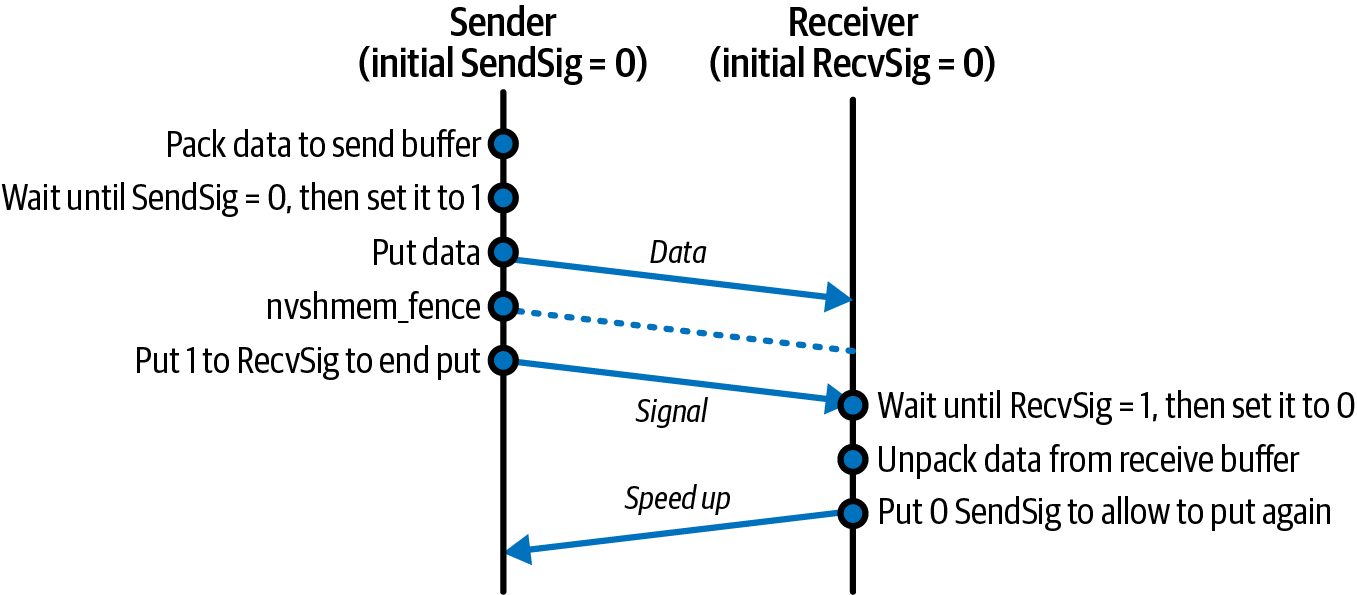
become a bottleneck if misused. NVSHMEM provides fine-grained primitives such as nvshmem_wait_until for waiting on device variables and signal operations like nvshmem_signal_fetch, nvshmem_signal_wait_until, or the nvshmemx_signal_op variants for point-to-point synchronization when only a subset of devices needs to coordinate. The low-level details showing NVSHMEM sharing data and synchroniz‐ ing with signals between a sender and a receiver GPU are shown in Figure 12-14.
Figure 12-14. NVSHMEM one-sided communication example
NVSHMEM shines when workloads are irregular or data-dependent, such as graph algorithms, dynamic load balancing, and discrete‐event simulations. In these cases, static graphs and collectives are not sufficient. Kernels that use NVSHMEM can be captured inside CUDA Graphs like any other kernel. The NVSHMEM device operations occur inside those kernels and are not separate graph nodes. However, NVSHMEM’s true strength is in letting kernels adapt and coordinate on the fly, without a fixed communication script used by a graph. In short, NVSHMEM transforms a cluster of GPUs into a shared‐memory domain, enabling device‐only kernel launches, data transfers, and synchronization at latencies and throughputs that far outpace any CPU‐mediated approach. Imagine a two-stage transformer inference pipeline (attention + multilayer percep‐ tron) that does the following: GPU 0 computes attention, then NVSHMEM puts its activations to GPU 1 and signals. GPU 1, running a persistent kernel, sees the flag and begins the MLP stage. Because GPU 0 immediately moves on to batch 2 while GPU 1 is still on batch 1, after a few iterations both devices are working in perfect tandem. Each handoff is hidden behind active compute warps. This drives near-100% utilization without incurring host stalls.
516 | Chapter 12: Dynamic Scheduling, CUDA Graphs, and Device-Initiated Kernel Orchestration
When you need flexible load balancing, NVSHMEM’s atomic operations let each PE
grab work dynamically. A PE is an OS process that is part of a parallel NVSHMEM
application.
The code here shows each GPU pulling the next index from a global counter, process‐
ing the chunk, then looping. This enables true work-stealing entirely on the device—
without host coordination:
    __global__ void work_steal_kernel(/*...*/, int *queue_head, Task *tasks) {
        while (true) {
            // Atomically claim the next task index
            int idx = nvshmem_int_atomic_inc(queue_head);
            if (idx >= N_tasks) break;
            // Process tasks[idx]...
        }
    }
For scenarios that require the lowest possible jitter, such as a tight multi-GPU collec‐
tive or synchronous model-parallel step, you can launch one cooperative kernel using
NVSHMEM and spanning all GPUs by using nvshmemx_collective_launch() to
start the sender and received kernels on GPU 0 and GPU 1 simultaneously. This
allows the to coordinate using NVSHMEM without any host intervention. Then, you
can use NVSHMEM’s device-side barriers, as shown here:
    __global__ void synchronized_step_kernel(/*...*/) {
        nvshmem_barrier_all();
        // All GPUs proceed in lockstep here
        // ...
    }
Here, every PE enters nvshmem_barrier_all() together and then continues simulta‐ neously. This guarantees perfectly aligned execution across the cluster.
               All kernels that use NVSHMEM’s device-level synchronization or
               collectives must be launched with nvshmemx_collective_launch().
               This ensures that the kernel runs concurrently on all PEs (GPUs) in
               the job.
Capturing Multi-GPU Collectives with NCCL and CUDA Graphs When you need bulk collective operations such as broadcasts, reductions, and all-to-all transfers, NVIDIA’s NCCL library is the go-to on multi-GPU systems. Traditionally, each GPU launches an ncclAllReduce or similar collective from the host. It then waits (synchronizes) before proceeding to the next compute phase. This sequential host orchestration adds overhead and idle time between the forward and backward passes.
Orchestrate Across Multiple GPUs and Cluster Nodes (NVSHMEM) | 517
However, NCCL calls can also be recorded into CUDA Graphs just like kernels. This
lets you “bake in” your forward kernels, the all-reduce, and your backward kernels
into a single graph that you replay each iteration:
      cudaStreamBeginCapture(captureStream,
          cudaStreamCaptureModeGlobal);
forwardKernel<<<...>>>(...);
      ncclAllReduce(sendBuf, recvBuf, count, ncclFloat,
          ncclSum, comm, captureStream);
backwardKernel<<<...>>>(...);
cudaStreamEndCapture(captureStream, &graph);
      // Instantiate and upload before launching
      cudaGraphExec_t graphExec;
      cudaGraphInstantiate(&graphExec, graph, ...);
      cudaGraphUpload(graphExec, captureStream);
// Each training step: cudaGraphLaunch(graphExec, captureStream); Notice the use of the same capture stream for all operations—including NCCL. Using a graph, NCCL calls become graph nodes just like kernels. Because each process is replaying an identical graph, NCCL’s internal logic finds peers and executes the allreduce without additional host coordination. This graph-captured all-reduce is espe‐ cially powerful on large clusters, as it eliminates per-iteration launch jitter and keeps all GPUs busy overlapping compute and network operations. Because each GPU launches the same graph, including its collective node, NCCL internally rendezvous across ranks without extra host intervention. The host’s periteration work drops to a single cudaGraphLaunch, which reduces CPU overhead and launch jitter. On top of reduced CPU load, capturing your all-reduce inside a graph allows true overlap of communication and computation across multiple GPUs and compute nodes. Suppose you split gradient computation into two passes, layers 1 through L/2 and layers (L/2 + 1) through L, and map them to separate streams, as shown here: // Pseudocode in capture: computeGradientsLayer1<<<...>>>(..., streamA); ncclAllReduce(..., comm, streamB); // in streamB, overlaps with streamA computeGradientsLayer2<<<...>>>(..., streamA); ncclAllReduce(..., comm, streamB); Since these nodes are captured with their unique stream assignments and dependen‐ cies, the CUDA driver can overlap NCCL’s network transfers on streamB with
518 | Chapter 12: Dynamic Scheduling, CUDA Graphs, and Device-Initiated Kernel Orchestration
independent work on streamA. This bucketed-all-reduce pattern consistently hides communication latency behind computation, improving multi-GPU scaling.
               NCCL collectives are graph capture–compatible when all ranks
               capture and replay the same sequence with the same communica‐
               tor. However, all ranks must capture and replay the same NCCL
               sequence with the same communicator. Mismatched communica‐
               tors across graph replays will risk deadlock (at best, relatively easy
               to debug) or incorrect results (at worst, silent failure, and difficult
               to debug). Also, it’s recommended to capture preliminary warmup
               collectives, run them ahead of time to initialize communicators,
               and reuse the instantiated graph to achieve minimal steady-state
               latency.
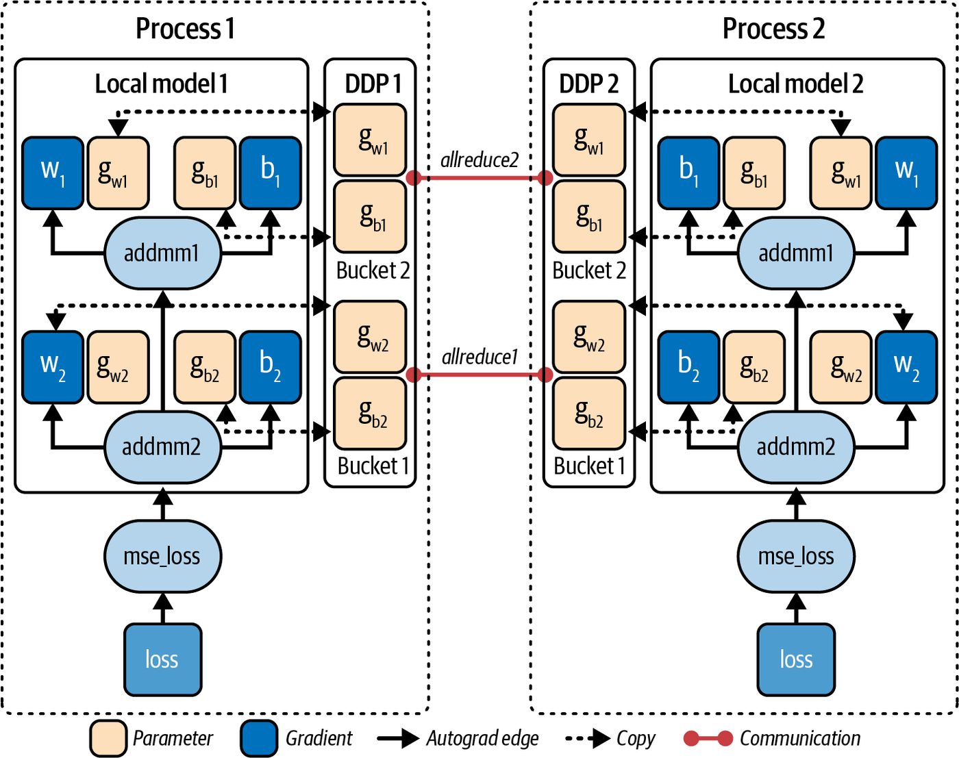
In practice, this bucketed all-reduce approach is standard in large-model training. By overlapping chunks of gradient reduction with computation of the next layers, you hide nearly all network time. An example of a bucketed all-reduce with DDP running in separate processes (process 1 and process 2) is shown in Figure 12-15.
Figure 12-15. Overlapping all-reduce with computation
Orchestrate Across Multiple GPUs and Cluster Nodes (NVSHMEM) | 519
Modern libraries like PyTorch DDP implement variants of this approach automati‐ cally. But capturing a CUDA Graph can further reduce CPU overhead and provide more deterministic performance. Keep in mind a few considerations for using CUDA Graphs in multi-GPU environ‐ ments. First, all participating GPUs must record and replay collectives in the identical sequence to avoid deadlock—much like MPI’s collective rules in which all ranks must enter the collective in the same order. Next, while CUDA Graphs pin and reuse GPU buffers, make sure allocations for your gradients and communication buffers are done before capture. Also, as discussed ear‐ lier, if you need to modify parameters in your graph, such as batch size, you can use cudaGraphExecUpdate to patch those parameters without a full recapture. In practice, capturing NCCL plus compute in a graph can cut per-step CPU time and speed up large-model training across many GPUs. At a massive scale, with hundreds of thousands of GPUs, these savings compound—creating tighter synchronization and higher utilization across the whole cluster.
                     NCCL and CUDA Graphs give us an efficient way to schedule col‐
                     lective communication alongside computation. However, not all
                     multi-GPU communication is collective—sometimes we need
                     more fine-grained or asynchronous sharing of data between GPUs.
                     This is exactly where NVSHMEM, described earlier, can help.
Pattern for N-GPU Scaling Whether you’re using simple peer copies, NCCL rings, or NVSHMEM one-sided atomics, the pattern of scaling to many GPUs is always the same. The system should dispatch kernels once, pipeline and overlap your data transfers with compute, and scale linearly—especially with the host CPU off the critical path. For example, 4 GPUs should ideally behave like a single GPU that is 4× faster— assuming you can keep all the GPUs fed with data in parallel (see Figure 12-16) and the host out of the loop. If you can do this, you should achieve near-linear speedups by properly overlapping communication computation. Without overlap, scaling will plateau once the communication time equals the computation time. As you increase GPUs, you need to use more aggressive pipelining of data transfers and computations—and use less CPU-side orchestration and synchronization. As such, you should offload more orchestration to the devices using asynchronous copies, NCCL collectives in graphs, and NVSHMEM’s PGAS primitives. This shifts even more responsibility to software.
520 | Chapter 12: Dynamic Scheduling, CUDA Graphs, and Device-Initiated Kernel Orchestration
Figure 12-16. Each GPU computes in parallel while exchanging data concurrently—no idle GPUs and no stalled data transfers
Applying these techniques, you can eliminate the CPU bottleneck, saturate the fast interconnects, max out the compute FLOPS, and build truly low-latency multi-GPU pipelines. Next, let’s revisit roofline models in the context of dynamic and device-side scheduling and orchestration.
Roofline-Guided Scheduling and Orchestration Decisions Over the last couple of chapters, we have collected a solid set of orchestration tech‐ niques, including CUDA streams, kernel fusion, persistent kernels, CUDA Graphs, dynamic parallelism, and more. The roofline model helps decide which tool will likely give the biggest win for your situation. At its heart, roofline boils down to operational arithmetic intensity, or the ratio of FLOPS performed to bytes moved. It consists of two hardware “ceilings”: memory roof (sloped) showing the peak throughput if you’re limited by bandwidth, and com‐ pute roof (flat) marking the peak arithmetic rate when you’re ALU‐bound, as shown in Figure 12-17. If your kernel lies near the memory roof (e.g., low FLOPS/byte) and is therefore memory bound, the best optimizations are those that hide or overlap memory trans‐ fers with computation. That means you should use asynchronous copies with CUDA streams—or even run multiple memory‐bound kernels concurrently. This way, you can better saturate different parts of the memory system.
Roofline-Guided Scheduling and Orchestration Decisions | 521
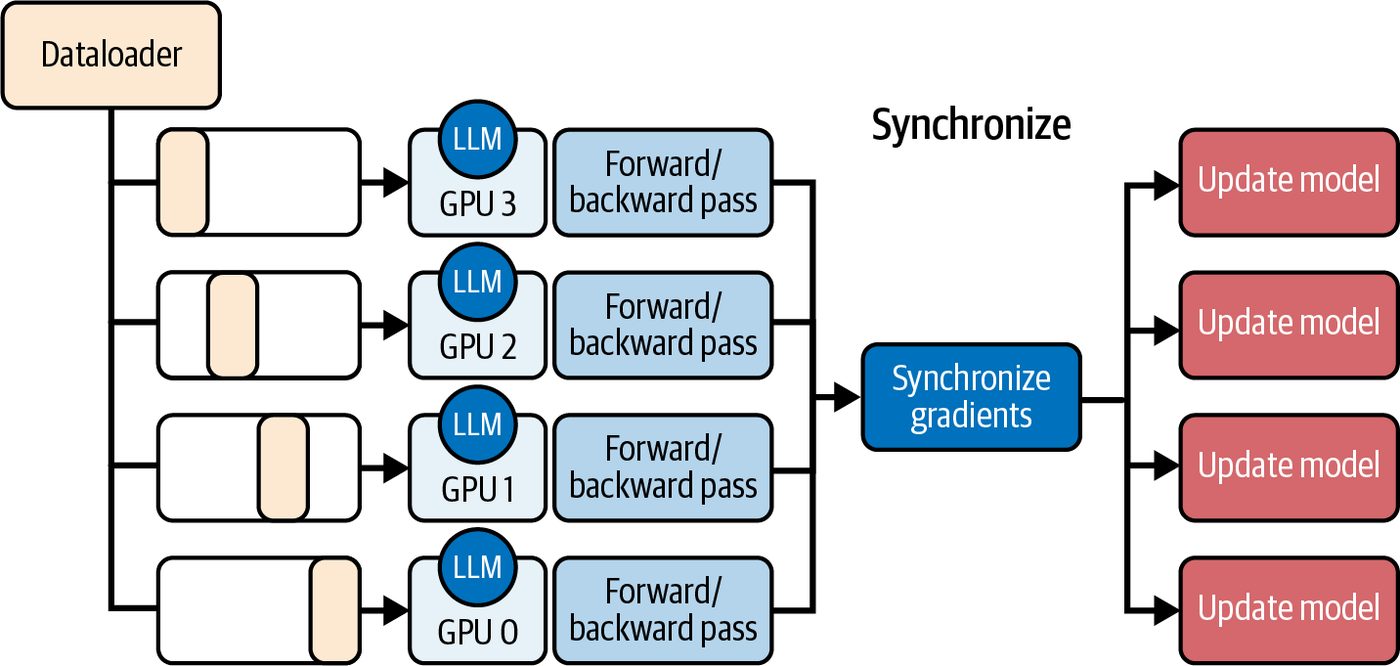
Figure 12-17. Arithmetic intensity with two hardware ceilings: memory bound (e.g., data transform operation) and compute bound (e.g., matrix multiply)
                    Kernel fusion helps only modestly for memory-bound workloads.
                    It can shave off a number of intermediate global‐memory round
                    trips. But the real gains come from masking latency and packing
                    more loads/stores in flight.
In contrast, a high‐intensity kernel sitting under the compute roof needs to keep its ALUs busy. Here kernel fusion shines by combining separate add+scale (our fused example from earlier) into one pass to increase FLOPS per byte, shift the point right‐ wards on the roofline plot, and push the kernel toward a higher percentage of peak FLOP/s. Likewise, persistent kernels, thread block clusters, and device‐initiated CUDA Graphs don’t change your intensity number, but they reduce idle gaps caused by repeated launches. This pushes your kernel’s performance closer to the flat compute ceiling. Many real workloads fall in between. They are neither strongly memory bound nor compute bound. In those cases, concurrency is your friend. By launching several modest‐intensity kernels in parallel, whether using streams, concurrent graphs, or multiple persistent kernels, you are combining them such that the aggregate‐ throughput point sits higher on both axes. This better utilizes the device’s resources. Thorough roofline analysis requires disciplined measurement. Use Nsight Compute to count FLOPS and bytes transferred, plot your kernel’s point, and see how far it lies below each roofline. If the workload is memory bound, reach for streams, overlap, and maybe reduce pre‐ cision (FP16, FP8, FP4) to reduce the denominator in the arithmetic intensity equa‐ tion (e.g., the number of bytes transferred.) And if your kernel is compute bound but not hitting peak FLOPS due to launch over‐ head or idle periods, focus on reducing launch overhead. As we’ve learned, you can do this by fusing operations into one kernel, using persistent kernels, capturing CUDA Graphs, or performing device-side launches. This will keep the ALUs fed.
522 | Chapter 12: Dynamic Scheduling, CUDA Graphs, and Device-Initiated Kernel Orchestration
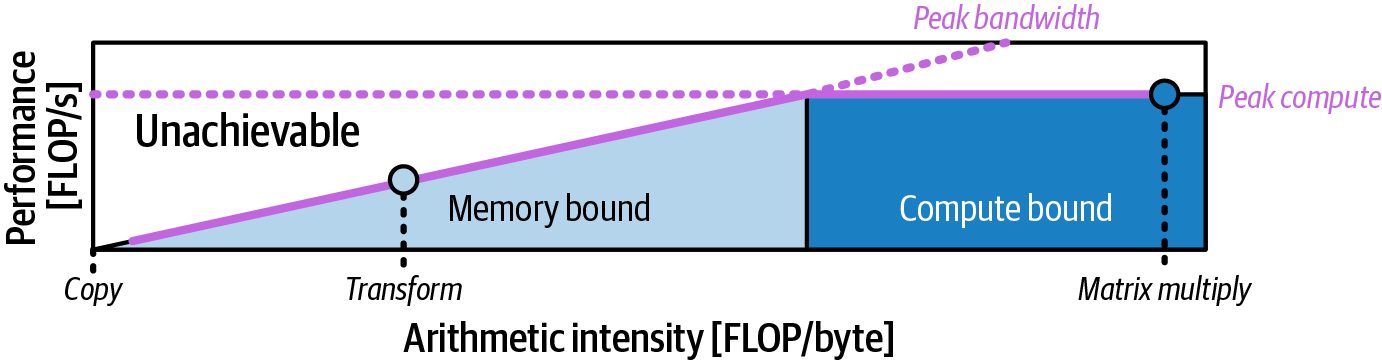
If your kernel sits well under both roofs and is neither fully memory nor compute bound, then try to increase concurrency. Run multiple kernels and streams in paral‐ lel. This will better utilize all of your system resources. With this quantitative guidance, you can pick the right orchestration strategy for your kernel rather than trying every trick all at once. Just remember to validate that each optimization moves you closer to the hardware’s true potential. Always measure after applying an optimization. The roofline model guides expectations, but real performance measurements, includ‐ ing compute throughput, achieved occupancy, memory throughput, etc., will tell the full story. A roofline analysis combined with iterative and continuous profiling will verify that your chosen optimization strategies are actually effective.
Key Takeaways Achieving peak GPU performance hinges on weaving together computation and data movement with minimal overhead. Efficient orchestration streamlines complex workloads across CPU and GPU, ensuring neither side stalls the other. Here are some key takeaways from this chapter: Dynamic scheduling with L2-cache atomic queues L2‐cache atomics on modern GPUs are exceptionally fast. Use fast L2-cache atomics with batched increments to balance irregular workloads on-GPU. This batched-work allocation reduces contention and keeps warps busy by eliminating warp idle gaps. It can significantly boost throughput up to ~2× in extreme imbal‐ ance cases but typically between 10% and 30%. Even a modest batch size of 8 or 16 can eliminate most contention due to the high L2 bandwidth. CUDA Graphs for fixed pipelines Record a sequence of GPU operations once and then replay it with a single host call each iteration. This reduces per-iteration CPU scheduling overhead, often a 20%–30% latency reduction (more at a larger scale). Make sure you’re achieving maximum overlap of dependent operations on the GPU. Low-overhead launch with CUDA Graphs Capture a sequence of asynchronous copies, kernel launches, event records, and allocations in a CUDA Graph (cudaStreamBeginCapture/cudaStreamEndCap ture). Replaying the graph with cudaGraphLaunch eliminates per-call CPU enqueue overhead while preserving all interstream dependencies, further reduc‐ ing runtime bottlenecks.
Key Takeaways | 523
Device-side orchestration
    Launch work from the GPU itself by tail-launching a prerecorded CUDA Graph
    or using dynamic parallelism to spawn child kernels. This eliminates CPU sched‐
    uling gaps entirely and allows the GPU to remain busy end to end with no host
    intervention.
Multi-GPU overlap
   Always overlap communication with computation. Use separate streams to pipe‐
   line GPU peer-to-peer transfers (cudaMemcpyPeerAsync), NCCL collectives,
   CUDA-aware MPI (RDMA), or NVSHMEM one-sided operations. This hides
   communication latency behind useful work and can approach linear scaling
   across many GPUs under favorable compute-to-communication ratios and ade‐
   quate overlap—and even across cluster nodes—when overlap is sufficient.
Roofline-guided choices
    Let the roofline chart drive your strategy. If your kernel is memory bound, focus
    on overlap and reducing data movement with asynchronous memcopies and
    mixed precision like FP8/FP4. If it’s compute bound but underachieving due to
    overhead, use launch-reduction techniques like kernel fusion, persistent kernels,
    and CUDA Graphs to approach the compute ceiling. For kernels in-between,
    increase concurrency by running multiple operations in parallel to utilize all
    hardware units. Always verify with profiling that the chosen optimization moves
    the needle.
By weaving these techniques together—dynamic dispatch, cooperative kernels, graph
capture/replay, and GPU-native memory sharing—you create pipelines that saturate
every part of the GPU cluster for ultrascale AI workloads.
Conclusion In this chapter, we moved beyond single-kernel optimizations and explored end-toend orchestration techniques. We covered how to launch work entirely on the device with dynamic parallelism, capture complex workflows in CUDA Graphs, and coordi‐ nate many GPUs using NCCL and NVSHMEM. Each technique shares the same goal: keep every engine fueled with work, hide latency, and collapse host–device gaps so that your hardware runs flat-out. NVIDIA’s modern GPU platforms blur the line between CPU and GPU more than ever. The Grace Blackwell and Vera Rubin Superchips, for example, connect the CPU with multiple GPUs using coherent NVLink with enormous bandwidth. But even as hardware reduces CPU-GPU barriers, the responsibility still falls on soft‐ ware to fully exploit this high-performance hardware. The approaches in this chapter, whether with CUDA in C++ or higher-level library APIs, are how we take advantage of these advancements.
524 | Chapter 12: Dynamic Scheduling, CUDA Graphs, and Device-Initiated Kernel Orchestration
In the next chapter, we’ll see how PyTorch integrates many of these ideas, including streams, graphs, asynchronous operations, and optimized kernels, so you can achieve this performance in just a few lines of Python. Let’s dive into the PyTorch ecosystem and understand why it’s so popular for implementing high-performance AI workloads.
Conclusion | 525