Ch 13 — Profiling, Tuning, and Scaling PyTorch
AI training and inference pipelines can suffer from performance bottlenecks at every layer, including Python interpreter overhead, CPU host-side data-loading stalls, CUDA kernel underutilization, and GPU device-memory contention. To optimize effectively, you need to profile at multiple levels of the stack using multiple tools that cover the entire system. This chapter focuses on profiling, debugging, and system-level tuning of PyTorch workloads running on modern NVIDIA GPUs. We will explore how to identify and fix bottlenecks using PyTorch’s built-in profiler, NVIDIA’s Nsight tools, and CPU profiling with Linux perf—as well as PyTorch memory profiling and memory alloca‐ tor tuning. We’ll also discuss how PyTorch uses CUDA streams for concurrency and CUDA Graphs to reduce kernel launch overhead. Next, we’ll show how to optimize data pipelines and scale out to multiple GPUs with PyTorch Distributed Data Parallel (DDP), Fully Sharded Data Parallel (FSDP), and other model parallelism strategies. We’ll then demonstrate how to profile multi-GPU and multinode environments, including Holistic Trace Analysis (HTA) and Perfetto. Throughout the chapter, we emphasize performance trade-offs and quantitative examples that focus on kernel execution times, hardware utilization metrics, memory footprint, data loading efficiency, and overall cost-efficiency of scaling. By the end of this chapter, you should have an understanding of how to implement an effective, holistic approach to profiling and tuning PyTorch workloads across the entire stack.
NVTX Markers and Profiling Tools To capture a holistic view of performance, it’s important to profile at multiple levels and use tools that cover the entire system. There exists a set of common tools and best practices used by practitioners and performance engineers to perform holistic profiling across all the layers in the system stack. Before we get to the tools, it’s important to highlight the NVIDIA Tools Extension (NVTX) and NVTX markers. These markers denote time ranges in a profiler’s time‐ line view and allow different profilers to correlate events across the same phases. For example, an NVTX range for "forward" will appear in both PyTorch profiler traces and Nsight Systems’ timelines. This makes cross-tool analysis much easier at different layers of the stack. NVTX markers are supported by most modern AI frame‐ works and libraries, including PyTorch and anything related to the CUDA ecosystem. NVTX markers are injected into code using either CUDA C++, PyTorch, or any C++ or Python library that supports NVIDIA GPUs (e.g., OpenAI Triton, PyCUDA, CuPy, cuTile, cuTe, CUTLASS, etc.). Most libraries already inject NVTX markers on your behalf for critical regions of code, such as "train_step", "forward", "backward", "optimizer_step", etc. But you can also inject them yourself using torch.pro filer.record_function() and torch.cuda.nvtx.range_push() in PyTorch, for instance. Now that we’ve described how to annotate interesting sections of your code using NVTX markers, let’s discuss the tools that can ingest, align, and visualize these mark‐ ers. Common profiling tools are summarized in Table 13-1 along with their scope, key features, and typical use cases. This table can help you choose the right tool for each stage of your optimization journey.
Table 13-1. Summary of profiling and visualization tools Tool Scope Features Typical use case PyTorch In-PyTorch opNVTX marker support, shape recording, memory Fine-grained breakdown of model profiler level profiling stats, trace export, identification of compile code; identify slow ops, GPU kernel (Kineto) (CPU/GPU) graph breaks launch overhead, or imbalance between forward/backward times. Nsight System-wide Unified timeline of CPU threads and GPU streams, End-to-end view of training/ Systems timeline (CPU, NVTX integration, multiprocess support inference pipeline; detect data (nsys) GPU, OS, I/O) loader stalls, CPU-GPU overlap issues, or inter-GPU synchronization delays. Nsight GPU kernel Per-kernel hardware metrics, source correlation, Deep dive into kernel efficiency Compute analysis (per roofline analysis, occupancy. and throughput after identifying hot kernels; (ncu) kernel) reports determine if a kernel is memory bound or compute bound, and why.
528 | Chapter 13: Profiling, Tuning, and Scaling PyTorch
Tool           Scope              Features                                            Typical use case
PyTorch        GPU memory         Memory snapshot timeline, per-op peak memory,       Diagnose fragmentation or
memory         usage by operation torch.cuda.memory_stats() and                       unexpectedly high memory usage.
profiler                          torch.cuda.mem_get_info() integration               See which ops allocate the most
                                                                                      memory and when, to optimize
                                                                                      memory footprint.
Linux perf CPU profiling and Sampling of CPU cycles/instructions/cache, flame Identify Python overhead
               system events      graphs, off-CPU (sleep) analysis                    (interpreter time, GIL contention),
                                                                                      CPU-side data loading bottlenecks,
                                                                                      or host OS scheduling issues.
Holistic Trace Distributed        Browser-based Kineto trace explorer, multiworker Analyze multi-GPU/multinode
Analysis       training trace     trace aggregation; incorporates Perfetto backend execution holistically. Find
               visualization                                                          imbalances or idle times, verify
                                                                                      overlap of communication with
                                                                                      computation.
Chrome         Offline trace      Web UIs for standard trace formats, advanced        Inspect traces without specialized
trace/         viewing (web-      filtering (Perfetto SQL engine), easy trace sharing software. It’s useful for performance
Perfetto       based)                                                                 dashboards or remote collaboration
                                                                                      on profiling data.
TorchEval      Model metrics and Standardized metrics API (throughput, accuracy, Log and monitor model
(metrics)      performance        etc.), easy integration                             throughput/latency alongside
               logging                                                                accuracy during training and
                                                                                      evaluation to correlate performance
                                                                                      with model quality.
ExecuTorch     Deployment         Model exporting, profiling, debugging, memory Use it to run PyTorch models and
               runtime for        analysis, visualization                             collect runtime metrics on
               mobile,                                                                constrained platforms, such as
               embedded, and                                                          mobile, embedded, and edge
               edge devices with                                                      devices, including Meta glasses, etc.
               lightweight
               profiling hooks
               and export tooling
Here is a detailed description of each profiling tool in Table 13-1: PyTorch profiler (Kineto) Within PyTorch, the torch.profiler, based on the Kineto open source project, provides operator-level breakdowns of CPU and CUDA/GPU runtimes. In addi‐ tion, it can record input shapes and take memory snapshots using simple Python context managers. The PyTorch profiler can capture detailed timeline traces and hardware counters across training and inference workloads using NVTX ranges to align the events. It provides end-to-end observability from Python code down to the CUDA kernels—and even provides performance tips for common issues like data-loading stalls and inefficient CUDA code.
NVTX Markers and Profiling Tools | 529
Nsight Systems (nsys)
    For system-wide correlation, including CPU threads, GPU kernels, OS events,
    I/O, and interconnect traffic, NVIDIA Nsight Systems produces a unified time‐
    line view. Its GUI and CLI reports can merge NVTX zones, Python call stacks,
    and CUDA streams across multiprocess and multinode runs. This makes it easy
    to spot where I/O and synchronization stalls might be impacting compute per‐
    formance.
Nsight Compute (ncu)
    Complementing Nsight Systems is NVIDIA Nsight Compute for per-kernel anal‐
    ysis. Nsight Compute collects detailed hardware metrics such as occupancy,
    memory bandwidth, and SM utilization. It can even generate roofline charts
    mapped to source code. Nsight Compute helps answer why a particular kernel is
    slow (e.g., memory bound, low occupancy) after other higher-level tools identify
    which kernels are the hotspots.
PyTorch memory profiler
   PyTorch also includes a memory profiler, which you can enable with pro
   file_memory=True in torch.profiler. The PyTorch memory profiler breaks
   down peak and cumulative GPU memory allocations per operation. This reveals
   memory usage hotspots that might otherwise go unnoticed.
Linux perf
    On the host side, Linux’s perf tool can sample CPU hardware counters, includ‐
    ing cycles, instructions, and cache misses—and unwind full C/C++ and Python
    call graphs. Starting with perf sched, you can see when CPU threads sit idle due
    to I/O or thread scheduling/synchronizing. This uncovers bottlenecks in data
    preprocessing loops, Python’s GIL, or synchronization that can starve the GPU.
Holistic Trace Analysis
    Meta’s open source Holistic Trace Analysis (HTA) tool ingests PyTorch profiler
    traces to help diagnose multi-GPU bottlenecks. With HTA, one can visualize dis‐
    tributed training timelines with NVTX ranges alongside CUDA kernel traces. By
    drilling into memory allocation patterns over time, you can identify periods of
    idle GPU—including when GPUs are waiting on each other.
                           TensorBoard’s PyTorch trace visualization plugin is depre‐
                           cated. Instead, use Perfetto for timeline viewing and Meta’s
                           HTA for distributed trace analysis.
530 | Chapter 13: Profiling, Tuning, and Scaling PyTorch
Chrome trace and Perfetto viewer
    For web-based exploration of large PyTorch profiler trace files, you can use
    Chrome tracing (e.g., chrome://tracing in the browser) and Perfetto UIs. These
    will load the JSON traces and let you interactively explore timeline views and
    flame charts. They even let you perform fine-grained filtering and SQL queries
    on the trace data—down to the submillisecond level for event tracing and corre‐
    lation. Chrome traces and the Perfetto UI are ideal for sharing profile results
    between members of your organization for cross-team analysis. (Note: Chrome’s
    legacy trace viewer is deprecated, so you should prefer the Perfetto web UI and
    SQL engine for viewing and analyzing traces.)
TorchEval (PyTorch’s metrics library)
    Another project, TorchEval, lets you log and monitor model throughput, latency,
    and quality metrics alongside training and evaluation metrics—all within a uni‐
    fied interface. TorchEval is PyTorch’s official metrics library and provides a sim‐
    ple API for end-to-end performance and quality metrics. This library makes it
    easy to plug into training loops and integrate across distributed environments.
ExecuTorch
    For embedded, mobile, and edge devices, the ExecuTorch project allows profil‐
    ing, visualizing, and debugging PyTorch models in lightweight runtime environ‐
    ments like Meta glasses. ExecuTorch has a small, dynamic memory footprint and
    supports Linux, iOS, Android, and embedded systems. Hugging Face supports
    ExecuTorch through its Optimum ExecuTorch project, which makes this envi‐
    ronment easy to integrate if you’re already using the Hugging Face ecosystem,
    like Hugging Face Transformers.
Next, let’s dive into an example of using these profilers to identify performance bot‐
tlenecks. We’ll then apply targeted optimizations and verify the performance
improvements.
Profiling PyTorch to Identify Bottlenecks Let’s profile an example mixture-of-experts (MoE) transformer model to see these tools in action. MoEs are LLMs with multiple expert layers—each expert is a feedforward network. Routing tokens to experts is managed by an expert gating system. We will run a single training iteration, capture detailed performance traces, and ana‐ lyze the output to guide our optimizations.
Profiling PyTorch to Identify Bottlenecks | 531
Using PyTorch Profiler First, we set up the model and input. We use Hugging Face Transformers to load the model and tokenizer, move the model to GPU, and prepare a small batch of inputs, as shown here: # train.py
      # Set up model and data
      model_name = "..."
      tokenizer = AutoTokenizer.from_pretrained(model_name)
      device = torch.device("cuda")
      model = AutoModelForCausalLM.from_pretrained(model_name).to(device)
      optimizer = torch.optim.AdamW(model.parameters(), lr=1e-4, fused=True)
      batch_size = 4
      input_texts = ["MoEs are great."] * batch_size
      enc = tokenizer(input_texts, return_tensors="pt", padding=True, truncation=True)
      input_ids = enc.input_ids.to(device)
      attention_mask = enc.attention_mask.to(device)
      labels = input_ids.clone() # For LM training, labels are the inputs
                                  # (next-token prediction)
To avoid capturing one-time setup costs, we run a few warm-up iterations before
profiling. This will prepare the model for analyzing and benchmarking by compiling
JIT kernels, filling caches, etc. This way, our measured iteration is representative of
steady-state performance. Here is the code to prepare the model:
      # Warm-up (not profiled)
      for _ in range(5):
          with torch.autocast(device_type="cuda", dtype=torch.bfloat16):
              outputs = model(input_ids, attention_mask=attention_mask, labels=labels)
          loss = outputs.loss
          loss.backward()
          optimizer.step()
          optimizer.zero_grad(set_to_none=True)
Now we profile one training iteration using PyTorch’s profiler and NVTX. We wrap the iteration in torch.profiler.profile() and mark high-level regions with record_function and NVTX ranges, including "forward", "backward", and "opti mizer_step", as shown here: from torch import profiler
      with profiler.profile(
          activities=[profiler.ProfilerActivity.CPU,
                      profiler.ProfilerActivity.CUDA],
          record_shapes=True, # record tensor shapes
          profile_memory=True, # track GPU memory usage per op
          with_stack=True,     # enable stack tracing
532 | Chapter 13: Profiling, Tuning, and Scaling PyTorch
        with_flops=True      # capture FLOPs counters
    ) as prof:
        with profiler.record_function("train_step"):
            # Forward pass
            torch.cuda.nvtx.range_push("forward")
            with torch.autocast(device_type="cuda", dtype=torch.bfloat16):
                outputs = model(input_ids, attention_mask=attention_mask,
                                labels=labels)
            loss = outputs.loss
            # end of forward
            torch.cuda.nvtx.range_pop()
            # Backward pass and optimization
            torch.cuda.nvtx.range_push("backward")
            loss.backward()
            torch.cuda.nvtx.range_push("optimizer_step")
            optimizer.step()
            # end of optimizer_step
            torch.cuda.nvtx.range_pop()
            optimizer.zero_grad()
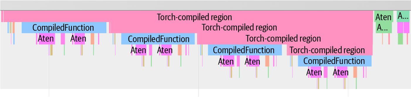
# end of backward torch.cuda.nvtx.range_pop() In this code, the PyTorch profiler is recording all CPU and GPU activities during the train_step. We use record_function("train_step") to define a top-level region. We also insert NVTX markers for the subphases ("forward", "backward", "opti mizer_step"). These markers will appear in profiler timelines to delineate phases of the iteration. The profiler can also highlight compiled versus noncompiled regions of the model. We’ll cover the PyTorch Compiler, graph breaks, and mechanisms to mitigate graph breaks later in this chapter—as well as the next chapter. For instance, when using torch.compile, the trace will show events like Compiled Function and indicate any graph breaks (see Figure 13-1). This helps pinpoint where the model fell back to eager execution, which will guide further optimizations.
Figure 13-1. Compiled (left and middle, pink) versus noncompiled (right, green) regions (source: https://oreil.ly/Z_fJG)
Profiling PyTorch to Identify Bottlenecks | 533
After execution, we can examine the operation-level results by calling prof.key_aver
ages().table() to print a concise table of the top operators by runtime. In the next
code block, we request the top 10 operations sorted by their self CUDA time, which is
the time spent in each operation’s own CUDA kernels excluding child operations
spawned by the kernel. The top 10 operations by CUDA execution time are summar‐
ized in Table 13-2:
      with profiler.profile(
          activities=[ProfilerActivity.CPU,
                      ProfilerActivity.CUDA],
          record_shapes=True,
          profile_memory=True,
      ) as prof:
          train_step(...)
      print(
          prof.key_averages()
              .table(
                  sort_by="self_cuda_time_total",
                  row_limit=10,
                  fields=["self_cuda_time_total",
                          "calls"]
              )
      )
Table 13-2. Profiler’s top 10 operations by CUDA execution time over one training iteration Operation Self CUDA total Calls aten::matmul 43.00 ms 128 aten::linear 35.50 ms 64 dispatch 18.70 ms 2 combine 12.10 ms 2 aten::layer_norm 10.20 ms 16 aten::softmax 5.70 ms 4 aten::scatter 4.10 ms 16 aten::gather 3.60 ms 16 aten::to 2.90 ms 8 aten::add_ 2.20 ms 64
Here, we see that the matrix multiplication operations (aten::matmul, and its use in aten::linear) dominate the CUDA time and consume the majority of the iteration. These operations correspond to the expert feed-forward network (FFN) GEMMs. Specifically, there are 128 calls to matmul per iteration. This makes sense since we
534 | Chapter 13: Profiling, Tuning, and Scaling PyTorch
have 64 experts—and each expert does a matmul in both the forward and backward passes. In Table 13-2, we see the next largest costs are from the dispatch and combine opera‐ tions. These are custom C++/CUDA kernels that redistribute tokens to experts—and then gather the outputs of the expert. The dispatch operation runs twice—once in the forward pass and once in the backward pass—for a total of 18.7 ms. The combine ran twice for 12.1 ms total. Together, these two operations account for another 30.8 ms of GPU time. The remaining time is spread across other smaller ops like layer norms, activations, etc. The key takeaway from this profiling example is that the expert FFN matmul is the top bottleneck, followed by the dispatch and combine kernels. Together, these dominate a training iteration’s runtime. To improve performance further, we should target those operations either by optimizing them directly or by reducing the number of times they’re called.
System Profiling with Nsight Systems and NVTX Timelines
The NVTX markers that we inserted make it straightforward to analyze the timeline
with Nsight Systems. To aggregate metrics per phase, we can profile the code using
nsys with an NVTX-based summary, as shown in the CLI command here:
    nsys profile \
       --output=profile \
       --stats=true \
       -t cuda,nvtx \
       python train.py
Here, the -t cuda,nvtx option instructs Nsight Systems to trace both CUDA API calls and NVTX ranges. After profiling, we can open the profile.nsys-rep file (--output=profile) in the Nsight Systems GUI or use the CLI to print the NVTX summary to the terminal. We can then use the CLI to generate the NVTX GPU Pro‐ jection Summary using one of the following commands on the profile.nsys-rep file, as shown here to validate ranges against projected GPU work with Nsight Systems: nsys stats --report=nvtx_gpu_proj_sum \ profile.nsys-rep
# or
    nsys recipe nvtx_gpu_proj_sum \
      profile.nsys-rep
You can use one of these commands in your continuous build and integration pipe‐
lines to monitor and detect any performance regressions. The results of this CLI
command are summarized in Table 13-3.
Profiling PyTorch to Identify Bottlenecks | 535
Table 13-3. NVTX GPU projection summary for one train_step iteration using Nsight Systems NVTX range GPU time (ms) Self GPU time (ms) Child GPU time (ms) Instances (calls) train_step 138.0 0.0 138.0 1 forward 60.5 60.5 0.0 130 backward 58.3 58.3 0.0 130 optimizer_step 19.2 19.2 0.0 1
Here, we see the train_step range includes the forward, backward, and optimizer subranges. This NVTX GPU Projection Summary confirms that the total GPU time under train_step is 138 ms. This time matches the sum of the forward, backward, and optimizer_step times from the PyTorch profiler output in Table 13-2. This shows consistency between tools. And although Table 13-3 shows a single optimizer_step call, its NVTX range actually brackets all 64 aten::add_ CUDA kernel launches (one add_ per expert as shown in Table 13-2) under the single optimizer_step marker. Note that Nsight Systems groups the 64 aten::add_ calls (e.g., 64-way expert parallel‐ ism strategy) into a single optimizer_step marker because it uses the CUDA Profil‐ ing Tools Interface (CUPTI) to capture NVTX push/pop events on the host. It then “projects” asynchronous GPU kernel execution times onto these CPU-defined inter‐ vals. As such, it sums the durations of every kernel with GPU start/end timestamps that fall between the corresponding push and pop calls. This produces one cumula‐ tive GPU time that exactly matches the total of the individual aten::add_ kernels.
                     Because NVTX markers have very low overhead when no profiler
                     is attached, this projection mechanism is ideal because it adds neg‐
                     ligible overhead while still providing end-to-end correlation of
                     GPU work with high-level code regions.
The forward and backward ranges each have self GPU time equal to their total time since we didn’t choose to nest deeper ranges inside of them. As such, child GPU time is 0 ms. However, train_step has nearly all of its time as child GPU time since it’s just a wrapper around the nested phases. The NVTX GPU projection summary also shows that, in each iteration, we observed 130 GPU activities inside train_step. These include kernel launches and other device operations such as memory copies, so they are not strictly one-to-one with kernels.
536 | Chapter 13: Profiling, Tuning, and Scaling PyTorch
As you can see in Table 13-3, the 130 GPU kernel calls happen for both the backward and forward passes as well. This one-to-one correspondence between operations and NVTX instances means that our instrumentation captures every important operation.
               The NVTX summary we show in Table 13-3 is a convenient text
               overview. For visual analysis, the timeline GUI can show overlap‐
               ping kernel execution, CPU thread states, and even CUDA API
               overhead events. In practice, you want to verify that host-side data
               loading and preprocessing are overlapping with GPU compute in
               the visual timeline. Any large gaps, or “bubbles,” indicate a prob‐
               lem. Small gaps for synchronization are expected and appropriate.
On a multi-GPU run, the Nsight Systems or HTA timeline view can reveal if NVLink or InfiniBand/Ethernet is being utilized effectively—or if a node is starved for work while waiting for communication or network delays. This would hint at suboptimal synchronization or load imbalance. It’s important to trace GPU communication events, including NCCL all-reduce calls and NVLink/NVSwitch activity using Nsight Systems and HTA to provide traces. These help verify that the GPUs stay busy in massive GPU domains such as an NVL72-based system. Careful profiling makes sure the system is using proper inter-GPU synchronization and balancing the workload in these large NVLink clusters. Let’s now zoom in on one of the most expensive kernels in the system: the matrix multiply, or matmul.
Kernel Roofline Analysis for General Matrix Multiply (GEMM)
To dive deeper and analyze the expert matmul, we invoke the CLI profiler Nsight
Compute (ncu) to target specific GEMM kernels by name. We’ll collect roofline-
related metrics to determine if it’s compute bound or memory bound, as shown here:
    ncu \
      --target-processes all \
      --kernel-name-regex "matmul" \
      --metrics \
        gpu__time_duration.avg, \
        gpu__dram_throughput.avg.pct_of_peak_sustained_elapsed, \
        lts__throughput.avg.pct_of_peak_sustained_elapsed, \
        sm__sass_thread_inst_executed_op_fp32_pred_on.sum, \
        sm__warps_active.avg.pct_of_peak_sustained_active \
      --csv full \
      -o matmul_roofline_report \
      python train.py
Here, we are collecting hardware counters for any kernel whose name matches “mat‐
mul”. Specifically, we collect a few key metrics, including GPU DRAM bandwidth and
Profiling PyTorch to Identify Bottlenecks | 537
L2 bandwidth as a percent of peak (gpu__dram_throughput.avg.pct_of_peak_ sustained_elapsed, lts__throughput.avg.pct_of_peak_sustained_elapsed), FP32 instruction count as a compute proxy (sm__sass_thread_inst_executed_op_ fp32_pred_on.sum), kernel time (gpu__time_duration.avg), and achieved occupancy (sm__warps_active.avg.pct_of_peak_sustained_active).
                      Metric identifiers can vary slightly across Nsight Compute releases.
                      If a metric is not found, use the UI to locate the current name and
                      substitute accordingly. Here, we are profiling SM and DRAM % of
                      peak sustained and achieved occupancy.
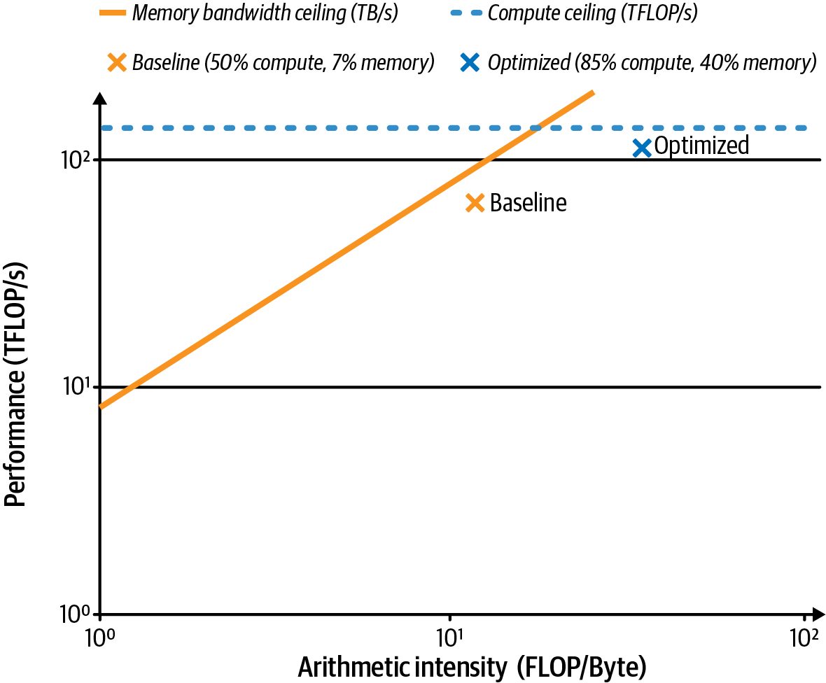
After applying the optimizations discussed until now, like reducing precision, fusing kernels, and increasing arithmetic intensity, we can rerun the ncu command to verify that our optimizations made a positive impact. Table 13-4 shows the comparison before and after applying these optimizations to improve arithmetic intensity.
Table 13-4. Roofline analysis for the expert matmul kernel before and after arithmetic intensity optimizations Kernel % of peak FLOPS % of peak memory BW Achieved SM Characteristic configuration (SM compute (memory throughput) occupancy throughput) Baseline 50% 70% 60% Memory bound (stalling on memory transfers) Optimized 85% 40% 80% Compute bound (near hardware roofline)
Here we see, in the baseline run, the primary GEMM kernel achieves only about 50% of peak compute FLOPS, 70% of peak memory bandwidth, and a moderate 60% SM occupancy (average active warps per SM). This occupancy is not enough to fully hide memory latency.
                      There is no universal occupancy target. Many high-performance
                      kernels achieve full latency hiding at 25–50% achieved occupancy.
                      Use Nsight Compute’s occupancy metrics together with stall‐reason
                      breakdowns and eligible warps per active cycle to judge whether
                      more occupancy would reduce stalls for the kernel. If the kernel
                      can’t schedule enough warps to cover the stall periods, this will lead
                      to idle cycles since memory requests aren’t being serviced quickly
                      enough.
The baseline metrics indicate a kernel that is memory bound since its execution is stalled by memory transfers. The result is a substantial amount of unused compute
538 | Chapter 13: Profiling, Tuning, and Scaling PyTorch
capacity, which further reinforces that this workload is not currently compute bound. The goal is to make this kernel more compute bound to take advantage of the large number of FLOPS available with this GPU. In the optimized version (e.g., fusing kernels, increasing arithmetic intensity, and reducing memory movement), the peak FLOPS increases to 85%, peak memory bandwidth drops to 40%, and occupancy increases to 80%. We effectively shifted the kernel from memory bound to compute bound—much closer to the hardware’s roof‐ line limits, as shown in Figure 13-2.
Figure 13-2. Roofline chart before and after increasing arithmetic intensity of this kernel
Up to this point, our profiling has focused on GPU performance. It’s also important to not waste time on the CPU or performing I/O. In the next section, we continue our profiling journey on the host side.
CPU and GPU Profiling with Linux perf To get a more holistic view of where time is being spent across both the host and device, we can use Linux perf to analyze CPU cycles, cache misses, branch misses, etc. We can then use these insights to drive a series of optimizations, apply them one by one, and measure the improvements.
Profiling PyTorch to Identify Bottlenecks | 539
First, let’s run a lightweight perf stat to gather CPU-side statistics during the MoE
training run on a node with an ARM-based Grace CPU paired with a Blackwell GPU.
Here is the CLI command followed by example output:
      perf stat -e \
        cycles,instructions,cache-misses,branch-misses \
        python train.py
          Performance counter stats for 'python train.py':
      # 0.600 CPUs utilized
      1,200.345 msec task-clock
      # Approximately 2.0 GHz
      2,400,567,890      cycles
      # 1.58 insn per cycle
      3,800,123,456      instructions
      # 0.32% of all cache refs
      12,345,678      cache-misses
      # 0.12% of all branches
      4,567,890      branch-misses
1.234567890 seconds time elapsed
This report from perf stat shows the CPU utilization, cycles, instructions per cycle (IPC), and cache/branch misses. In our run, the task clock shows ~1.2 seconds with only ~60% (0.600) of a single CPU core used over the measured interval. This is expected, as the GPU is doing most of the heavy lifting. The low cache-miss and branch-miss rates hint that memory access patterns and branch prediction were rela‐ tively efficient on the CPU side for this workload. However, the instructions per cycle (IPC) measurement of just 1.58 shows that the CPU is issuing well below the eight instructions per cycle theoretical maximum IPC for a single Grace CPU core (ARM Neoverse V2). This indicates potential inefficiencies such as memory latency, I/O stalls, or host-compute issues in this specific workload. We can explore further using perf record and perf report to pinpoint which Python and C++ functions dominate the CPU execution time during training. These CLI commands are shown here: perf record -F 2000 -g --call-graph dwarf -o perf.data \ python train.py
Here, we use perf record to collect samples at 2000 Hz (-F 2000) and capture full C/C++ and Python call stacks by specifying -g --call-graph dwarf. DWARF stands for Debugging With Attributed Record Formats, and it’s a standard debugging data format embedded in compiled binary files (e.g., ELF files). The DWARF output trace is saved to perf.data (-o perf.data). We then use perf report to generate a sum‐ mary report of the hottest call stacks and their sample percentages:
540 | Chapter 13: Profiling, Tuning, and Scaling PyTorch
perf report --stdio -n -g -i perf.data
    # Samples Command   Shared Object       Symbol
    # ........ ........ ................... .................................
         45.0% python    python              py::forward <...> /src/train.py
         20.5% python    python              aten::matmul
         10.2% python    python              dataloader_iter_next
          8.7% python    libnccl.so          ncclAllReduce
          5.3% python    libc.so.6           read
          ...   ...      ...                 ...
Here, we see that the Python interpreter’s forward function, the Python side of our training loop, accounts for 45.0% of CPU samples. PyTorch’s C++ aten::matmul operation accounts for 20.5%, the DataLoader’s iterator next function for 10.2%, an NCCL all-reduce call for 8.7%, and I/O reads for 5.3%. These percentages tell us where to invest our optimization effort. Based on this pro‐ file, we address each bottleneck with a specific mitigation plan to improve perfor‐ mance of our system: Excess Python overhead (45% in py::forward) Use PyTorch’s JIT compiler using torch.compile (discussed in the next section) to eliminate interpreter overhead and fuse Python-side operations into optimized CUDA code. Large matmul hotspot (20.5% in aten::matmul) Either use the PyTorch Compiler to optimize this code or move this critical matrix multiply into a custom CUDA C++ kernel (e.g., fused kernel) to bypass Python and use the optimized CUDA code directly. Data loading stalls (10.2% in dataloader_iter_next) Increase PyTorch’s DataLoader num_workers. A common guideline is one worker per CPU, but you can experiment with more to find the right level of I/O parallelization. Just make sure you don’t oversubscribe the CPU cores. You should also enable persistent_workers=True so that worker processes stay alive across epochs and avoid startup overhead for each epoch. Fuse or parallelize multiple torch.utils.data.DataPipe. This can reduce Python overhead in complex data pipelines. Gradient synchronization overhead (8.7% in ncclAllReduce) Optimize multi-GPU communication. For instance, you can increase the gradi‐ ent bucket size in DistributedDataParallel. It’s common to increase the bucket_cap_mb from 25 MB to 50 MB so that NCCL can launch all-reduce oper‐ ations sooner and overlap them with backward computations. You can also con‐ sider gradient compression techniques or NVIDIA’s NCCL compression for 8-bit gradients to reduce bandwidth usage. These may incur a slight cost to accuracy.
Profiling PyTorch to Identify Bottlenecks | 541
Host I/O bottleneck (5.3% in read syscalls)
    Use pinned memory (pin_memory=True) and nonblocking GPU copies
    (.to(device, non_blocking=True)) in the DataLoader to overlap CPU-to-GPU
    data transfers. Also, you can batch file reads or bundle many small files into an
    optimized dataset format like Arrow, WebDataset (tar shards), TFRecord, or Par‐
    quet chunks that facilitate large sequential reads. It’s best to prefer contiguous
    shard formats over per-sample files. Prefer pinned host buffers when using a
    larger prefetch depth (e.g., prefetch_factor=4 or 8). Combined with persis
    tent_workers=True, your system will keep loader threads busy since compute-
    communication are overlapping efficiently. This will eliminate per-file overhead
    when reading many small files in large corpora.
These approaches, combined with large OS read-ahead and NVMe SSDs, will boost
I/O throughput. Also, newer filesystems and storage libraries like NVIDIA Magnum
IO can help pipeline data efficiently to the GPU.
After formulating this plan, you should systematically apply each optimization and
measure the effect. Remember to implement and test these optimizations one by one
to verify that each actually improves performance. This helps avoid situations in
which multiple changes interact in unexpected ways. By isolating each change, you
know which adjustments have a positive effect and which do not.
On systems with the NVIDIA Performance Monitoring Unit (PMU) drivers present,
you can use perf to sample NVIDIA chip interconnect and fabric counters alongside
CPU counters, including NVLink-C2C devices exposed under /sys/bus/
event_source/devices as nvidia_nvlink_c2c*, for instance. Verify availability with
perf list and by checking the nvidia_pmu entries under sysfs.
                     Linux perf for NVIDIA PMUs is limited to device-level link and
                     fabric events such as NVLink-C2C on Grace-Blackwell. SM pipe‐
                     line, warp stall, and memory throughput counters remain CUPTI
                     and Nsight tools only. These PMUs do not expose SM-level kernel
                     metrics. For SM utilization, occupancy, and memory throughput,
                     use Nsight Compute or a CUPTI-based profiler. Make sure to set
                     NVreg_RestrictProfilingToAdminUsers=0 to allow non-root
                     profiling of SM-level hardware counters.
Once the PMU devices are present, you can collect CPU and NVIDIA events together. Use symbolic event names reported by perf list: perf list | grep -i nvidia
      perf stat -a \
        -e nvidia_nvlink_c2c0_pmu_0/cycles/ \
        -e cycles,cache-misses \
        python train.py
542 | Chapter 13: Profiling, Tuning, and Scaling PyTorch
Here, the cycles event on the NVLink-C2C PMU lets you correlate GPU interconnect activity with host CPU behavior. The following is example output from the preceding perf stat command, which shows the NVLink C2C PMU recorded activity during the run while the CPU incurred cycles and cache misses: Performance counter stats for 'python train_deepseek_v3.py':
          3,567,890,123 nvidia_nvlink_c2c0_pmu_0/cycles
             45,678,901 cycles
              7,890,123 cache-misses
2.345678901 seconds time elapsed Our initial profiling revealed that GPU compute (e.g., expert matrix multiplies) and GPU communication (e.g., dispatch and combine operations) are the primary bottle‐ necks based on the PyTorch profiler and Nsight tools. However, CPU, data loading, and GPU collective communication operations also impact performance as perf demonstrates by showing which CPU threads and interconnect PMUs are active dur‐ ing the slow regions.
               To dig into additional link and fabric request counters, pick addi‐
               tional NVIDIA PMU events that appear on your system from perf
               list and add them to the perf stat command, as shown
               previously.
In short, by combining high-level CPU throughput metrics and call graph hotspots from perf with device metrics and timelines from Nsight Systems and Nsight Com‐ pute, you can build a holistic performance story across host and device. Start by addressing the largest CPU-side bottlenecks and data stalls. Next, optimize GPU communication and tune the GPU kernels.
PyTorch Compiler (torch.compile) One of the quickest wins in PyTorch is to use the PyTorch compiler with torch.com pile(). The compiler stack includes TorchDynamo, AOT Autograd, and TorchIn‐ ductor, which capture graphs, fuse ops, and generate high-performance code for the target backend (e.g., NVIDIA GPUs). The PyTorch Compiler can eliminate a lot of Python interpreter overhead and GPU kernel launch latency by fusing together many small operations into larger kernels. After doing our baseline profiling, we enabled torch.compile on the model to see if we could get an easy speedup. Next, let’s describe this process—and the results.
PyTorch Compiler (torch.compile) | 543
Using the PyTorch Compiler Using the PyTorch compiler with the default settings is straightforward and requires no code changes besides wrapping the model as shown here: model = torch.com pile(model). Under the hood, TorchDynamo traces the Python code, AOT Autograd captures the backward pass, and TorchInductor, which leverages OpenAI’s Triton for GPU kernel code generation (as discussed in the next chapter), produces efficient fused kernels automatically. The compiler observes our model’s forward pass and identifies many opportunities to fuse consecutive operations, such as elementwise activations, layer norms, etc. It gen‐ erates fused kernels for those operations—and also for parts of the backward pass. The result is significantly fewer kernel launches and less CPU overhead per iteration. The compile step does introduce some overhead on the order of seconds—or even minutes for very large models—but this cost is amortized over long training jobs or repeated inference runs. Fortunately, TorchInductor caches compiled kernels so that subsequent runs don’t pay the compile cost again. The PyTorch community is also continuously working to improve compile/startup performance by allowing you to save and reuse compiled artifacts across runs. Use torch.compiler.save_ cache_artifacts() and torch.compiler .load_cache_artifacts() to persist TorchInductor outputs across runs or nodes. This reduces startup on long-running training or serving. One example is the PyTorch Mega-Cache feature. This is an end-to-end compile cache that lets you save compiled kernels to disk and reload them in future runs. With PyTorch Mega-Cache, you can compile once (e.g., offline) and reuse the opti‐ mized kernels across multiple training sessions. This helps to reduce startup time. You’ll still benefit from TorchInductor’s kernel optimizations like warp specialization, but you’ll avoid recompiling the graph each time.
                     You can even use this compile cache on other compute nodes. If
                     you do this, make sure CUDA, PyTorch, and Triton versions are
                     compatible across the nodes.
It’s worth noting that PyTorch’s Compiler applies sophisticated optimization tech‐ niques internally. For example, we mentioned warp specialization in Chapter 10. TorchInductor’s autotuner generates multiple kernel variants across tile sizes, mem‐ ory access patterns, etc. It will apply techniques like memory-warp versus computewarp specialization behind the scenes. It will then choose the fastest variant for your hardware automatically.
544 | Chapter 13: Profiling, Tuning, and Scaling PyTorch
TorchInductor supports prologue and epilogue fusion around GEMM kernels. For example, bias-add comes before the matmul. And, after the matmul, the epilogue con‐ sists of elementwise operations such as activation, dropout, and residual. By merging these kernel prologue and epilogue operations into a single optimized kernel, TorchInductor reduces memory traffic, minimizes kernel-launch overhead, and increases occupancy. You can verify this with the profiler, which will show higher SM utilization. This optimization complexity remains entirely transparent to the developer since PyTorch presents a clean, tensor-centric interface without exposing CUDA-level warp details. So while you won’t see “memory warp” or “compute warp” flags in the PyTorch API, just know that these techniques are being used under the hood. Once the code is compiled, you will notice the benefits of warp specialization in profiler metrics, including higher occupancy, fewer memory latency stalls, and increased SM utilization. To illustrate the benefit of a compiled mode, let’s compare PyTorch’s eager mode ver‐ sus compiled execution on an MoE model. We’ll time a single training iteration of the model in regular eager mode and then again with the "max-autotune" compiled mode. The code is shown here, followed by the example output: import torch from transformers import AutoModelForCausalLM, AutoTokenizer
    # ---- Setup Model ----
    device = 'cuda'
    model_name = "..."
    tokenizer = AutoTokenizer.from_pretrained(model_name)
    model = AutoModelForCausalLM.from_pretrained(model_name).to(device)
    optimizer = torch.optim.AdamW(model.parameters(), lr=1e-4, fused=True)
    # ---- Create a dummy batch of token IDs ----
    batch_size = 4
    input_texts = ["MoE's are awesome!"] * batch_size
    enc = tokenizer(input_texts, return_tensors="pt", padding=True, truncation=True)
    input_ids = enc.input_ids.to(device)
    attention_mask = enc.attention_mask.to(device)
    labels = input_ids.clone() # for causal LM, labels = input_ids
    # ---- Make runs deterministic ----
    torch.backends.cudnn.benchmark = False
    torch.backends.cudnn.deterministic = True
    # --- Eager timing ---
    torch.cuda.synchronize()
    start = torch.cuda.Event(enable_timing=True)
    end = torch.cuda.Event(enable_timing=True)
for _ in range(iters_warmup):
PyTorch Compiler (torch.compile) | 545
           out = model(input_ids, attention_mask=attention_mask, labels=labels)
           loss = out.loss if hasattr(out, "loss") else out
           loss.backward()
           optimizer.step()
           optimizer.zero_grad(set_to_none=True)
      torch.cuda.synchronize()
      start.record()
      for _ in range(iters_meas):
          out = model(input_ids, attention_mask=attention_mask, labels=labels)
          loss = out.loss if hasattr(out, "loss") else out
          loss.backward()
          optimizer.step()
          optimizer.zero_grad(set_to_none=True)
      end.record()
      torch.cuda.synchronize()
      print(f"Eager mode step time: {start.elapsed_time(end)/iters_meas:.3f} ms")
      # --- Compile the model (choose one mode)
      # enables graph trees
      compiled_model = torch.compile(model, mode="reduce-overhead")
      # Alternatives:
      # more tuning, longer compile
      # compiled_model = torch.compile(model, mode="max-autotune")
      # balanced
      # compiled_model = torch.compile(model, mode="default")
      # Warm-up compiled
      for _ in range(iters_warmup):
          out = compiled_model(input_ids, attention_mask=attention_mask, labels=labels)
          loss = out.loss if hasattr(out, "loss") else out
          loss.backward()
          optimizer.step()
          optimizer.zero_grad(set_to_none=True)
      torch.cuda.synchronize()
      start.record()
      for _ in range(iters_meas):
          out = compiled_model(input_ids, attention_mask=attention_mask, labels=labels)
          loss = out.loss if hasattr(out, "loss") else out
          loss.backward()
          optimizer.step()
          optimizer.zero_grad(set_to_none=True)
      end.record()
      torch.cuda.synchronize()
      print(f"Compiled mode step time: {start.elapsed_time(end)/iters_meas:.3f} ms")
In this case, PyTorch eager mode takes roughly 248 ms per iteration. After warming
up and letting the compiler perform its optimizations, the compiled mode runs in
about 173 ms. Our compiled version, using "max-autotune", runs ~30% faster than
eager execution. Actual speedup varies with model structure, batch size, and dynamic
546 | Chapter 13: Profiling, Tuning, and Scaling PyTorch
shapes. Dense models dominated by a single large GEMM may only see <10% speedup. These savings come primarily from combining many small GPU kernels. Small GPU kernels are common in an MoE architecture for token dispatch/combine and pertoken activation patterns. By fusing these small operations into fewer, larger kernels, we keep intermediate data in faster on-chip memory—such as registers and shared memory—rather than repeatedly moving data to and from global device memory (HBM).
               For highly dynamic token routing used by MoE architectures, pre‐
               fer default or max-autotune-no-cudagraphs. Then switch to max-
               autotune once input shapes stabilize—or when you use CUDA
               Graph Trees with limited discrete shapes.
In this case, many of the small operations, like dispatch/combine, activation func‐ tions, etc., are fused away by TorchInductor. If you examine the trace of the compiled run, you’ll see far fewer GPU kernels on the timeline. Instead, there will be fewer, but slightly longer-running, kernels that correspond to merged operations performing multiple steps at once. Over many iterations, the benefit is even more pronounced as the one-time compila‐ tion overhead is amortized. Profiling the compiled model’s execution shows far fewer GPU kernel launches, as many operations that were separate in eager mode are now fused together. It’s worth noting that if a dense model is dominated by one massive GEMM due to a large linear layer, for example, it may see only modest gains (e.g., < 10%) from torch.compile. This is because the model is likely using Tensor Cores efficiently— and because there is little opportunity for kernel fusion and Python overhead removal. However, sparse architectures like MoE, with hundreds of medium-sized matmul operations, will see big wins since compilation reduces Python overhead, lowers ker‐ nel launch latency, and fuses multiple steps into optimized kernels. As such, the PyTorch compiler leads to significantly larger performance gains for MoEs compared to dense models. In addition to automatic operator fusion, you can integrate user-defined custom ker‐ nels directly into the torch.compile workflow. This approach combines the best of both worlds since it uses compiler-managed graph-level optimizations for general patterns while giving you full control when needed. For instance, you can write a specialized Triton or CUDA kernel for a performancecritical operation and register it as a custom operator. When the model is traced and
PyTorch Compiler (torch.compile) | 547
compiled, TorchInductor will treat it as a single fused operation within the larger exe‐ cution graph. The result is a combination of custom hand-tuned code embedded in a fully optimized, compiler-managed execution graph. TorchInductor’s flexibility lets your custom kernel benefit from the compiler optimiz‐ ing the surrounding operations (e.g., fusion with adjacent layers, etc.). In practice, this means you can use your own high-performance kernel without losing PyTorch compiler’s ability to optimize the rest of the model. In short, by using PyTorch compile, including its "max-autotune" mode within our training loop, you can get decent speedups on modern GPUs with relatively low effort. This can be verified holistically using torch.profiler, Linux perf, Nsight Sys‐ tems, Nsight Compute, and other helpful profilers.
Compiling Versus Writing Custom Kernels With a compiler backend like TorchInductor, many operations will be fused into effi‐ cient kernels automatically. As we saw, simply using torch.compile gives a decentsized boost with minimal effort. However, there may be times when the automatically generated code is not as optimal as a custom-crafted kernel—or when an operation isn’t captured by the compiler at all. This raises the question: when should you rely on the compiler’s fusion versus writing a custom CUDA kernel yourself? For most cases, using high-level torch.compile with graph capture—and TorchIn‐ ductor under the hood—is preferred. This is much less effort than writing custom CUDA kernels—and often produces good enough performance improvement without specialized coding. TorchInductor already applies many advanced optimizations internally, such as fusion of elementwise operations, merging of layer operations, layout optimization, etc. Writing fused kernels by hand would be time-consuming and brittle, whereas the compiler can do these automatically in most cases. If your model uses a novel operation or pattern that the compiler doesn’t handle well, you may need to write a custom kernel and integrate a custom operator with PyTorch. In the next chapter, you’ll see how to do this in more detail. In short, use torch.compile as the first resort for performance tuning since it’s easy, sufficient, and relatively “free.” Creating custom kernels is the next level of optimiza‐ tion and is used when built-in automation isn’t enough. Only after that should you consider writing custom kernels for the remaining hotspots to fuse certain unsupported optimizer operations or specialized attention patterns. However, even for specialized attention patterns, PyTorch provides the FlexAttention API (prefill) and FlexDecod‐ ing API (decode), which are the preferred ways to implement custom attention kernels in PyTorch for training and inference, as we’ll see in an upcoming section.
548 | Chapter 13: Profiling, Tuning, and Scaling PyTorch
Compilation Modes and Trade-Offs in Speed, Memory, and Compile Time PyTorch provides several modes for torch.compile that tune the compiler’s aggres‐ siveness and capabilities for different scenarios. You can explicitly select a mode using torch.compile(model, mode="..."). The choices are "default", "reduceoverhead", "max-autotune", and "max-autotune-no-cudagraphs". Each mode pro‐ vides a combination of options regarding CUDA Graphs, autotuning, and optimization level. The modes are summarized in Table 13-5.
Table 13-5. Summary of compilation modes and their key characteristics
Mode           Description                                       Compile      Extra memory Notable features
                                                                 time
default        Balanced optimizations (good speed without        Low–         No              General fusion, basic
               long compile or extra mem); includes minor        Medium                       autotuning
               autotuning; may use CUDA Graphs for stable
               segments
reduce-        Reduces per-iteration overhead (good for small    Medium       Yes             Uses CUDA Graphs (if
overhead       batches); ideal for inference or small batches;                (workspace      possible) to eliminate
               automatically skips CUDA Graphs if it detects                  caching)        launch overhead
               dynamic shapes to preserve correctness
max-           Maximizes runtime performance (best for long      High (slow Maybe (if         Aggressive Triton
autotune       runs); longer compile time; best for aggressive   compile)   graphs are        autotuning; enables
               tuning for a large amount of SMs and GPU                     used)             CUDA Graphs on GPU
               memory
max-           Does everything max-autotune does but             High         No              Same as max-
autotune-      without CUDA Graph capture                                                     autotune but
no-            Best for dynamic shapes or for debugging issues                                disables graphs for
cudagraphs     masked by CUDA Graphs                                                          flexibility
Here’s a detailed description of the modes in Table 13-5:
default
    This is the default mode if no mode is explicitly specified. This mode provides a
    balance of reasonably fast compiled code without excessive compile time or
    memory usage. It will do standard optimizations and use the default TorchInduc‐
    tor backend. This mode is often best for large models where compile time needs
    to be moderate—or when memory is tight. This mode includes minor autotuning
    and may use CUDA Graphs for stable segments. But it tries to balance speed and
    compile-time cost.
PyTorch Compiler (torch.compile) | 549
reduce-overhead
      This mode focuses on minimizing Python and runtime overhead. This is espe‐
      cially useful for small models—or models that perform a short number of execu‐
      tions per iteration. In these cases, even a little bit of overhead hurts performance.
      This mode leverages CUDA Graphs aggressively to eliminate per-iteration launch
      overhead. It may also allocate some extra memory for persistent use, such as
      workspace memory that is reused. This avoids frequent CUDA malloc and free
      calls. For example, it might cache a large working tensor instead of allocating it
      each iteration. This mode will automatically skip CUDA Graphs and fall back to
      eager if it detects dynamic shapes. It does this to preserve correctness.
      This mode can speed up inference and training in low-latency scenarios—at the
      cost of some additional memory. Note that CUDA Graphs require that the graph’s
      memory addresses stay constant, so this mode can be used only when input sizes
      do not change and certain operations, such as dynamic-shape operations, are not
      present. Otherwise, graphs would break or be recompiled. The compiler will auto‐
      matically fall back if it can’t apply a CUDA Graph in a given segment.
max-autotune
      This mode generates the fastest possible code without regard for compile time. It
      will run extensive autotuning of kernels by trying many tiling configurations for
      matrix multiplications, for instance, and utilize any known performance opti‐
      mizations in TorchInductor. On modern GPUs, max-autotune also enables
      CUDA Graphs by default for stable execution.
      The compilation process in this mode can be significantly longer—on the order
      of minutes for a large model. It’s intended for scenarios in which you compile
      once and run the model many times, such as running long training jobs or
      deploying a model that will handle a lot of requests over time. In exchange for
      long upfront compile times, you often get the best runtime performance. For
      instance, after automatic tuning, your matmuls might run with an optimal block
      size for your specific GPU and tensor shapes. This gives this mode an edge over
      default heuristics.
max-autotune-no-cudagraphs
      As the name suggests, this mode is the same as max-autotune but with CUDA
      Graph capture disabled. This is important for cases in which CUDA Graphs
      interfere with desired runtime behaviors that are not compatible with CUDA
      Graphs. For instance, since CUDA Graphs require static shapes and memory
      addresses, you can’t use varying input shapes or rely on allocating new memory
      for each iteration.
      Also, when measuring performance, using CUDA Graphs can mask the overhead
      of launching kernels, which might not be desired in some benchmarks. So this
550 | Chapter 13: Profiling, Tuning, and Scaling PyTorch
mode allows maximal kernel optimization without CUDA Graphs. This will help maintain flexibility and allow you to debug any issues that CUDA Graphs might introduce (or mask), such as shape-dependent control flow or occasional alloca‐ tor readdressing during graph capture. Use this mode when input sizes vary each iteration—or for debugging issues that might be masked by the use of CUDA Graphs. For most use cases, the default mode is a good start. It’s meant to give sizable speed‐ ups with minimal hassle. If you find that your model still isn’t fast enough and you can tolerate longer compilation, try reduce-overhead and max-autotune for poten‐ tially better fused kernels—especially if your model is dominated by large matmul operations that can be autotuned. max-autotune can sometimes regress latency on some models. Be sure to profile the different modes for your specific workload and hardware. On the other hand, if you are optimizing a very small model or a portion of code where Python overhead is the bottleneck, such as a tight training loop with lots of small tensor operations, using reduce-overhead can produce the best gains by removing virtually all kernel-launch runtime overhead using CUDA Graph capture. Just be mindful of the constraints of reduce-overhead. It works best when the work‐ load per iteration is consistent and fits the graph-capture requirements, including no dynamic shape changes, no new memory allocations, etc. The max-autotune-no-cudagraphs mode is more of a specialized option. It’s useful if you want maximum kernel optimization but either cannot use graphs due to varying input sizes or want to measure raw kernel performance without graph amortization. In all cases, it’s wise to profile and measure after changing the PyTorch compiler mode. The different modes exist because one size doesn’t fit all in performance engi‐ neering. Furthermore, you should monitor memory usage when choosing a mode. Modes that use CUDA Graphs will allocate large, static buffers that increase memory footprint. For extremely memory-constrained cases, you might prefer this no-graphs mode to avoid the extra memory overhead of CUDA Graphs. Next, let’s discuss how to inspect what the compiler is doing, including whether it created one graph or many—or whether it used CUDA Graphs, etc.
Regional Compilation For models with many identical blocks, such as Transformers and MoEs, you can use regional compilation to decrease cold-start execution time. Additionally, it’s useful to reduce recompilation churn—all without sacrificing the power of kernel fusion. Specifically, regional compilation reduces compile time by compiling the repeated block (e.g., a Transformer block) once and reusing that code across all occurrences.
PyTorch Compiler (torch.compile) | 551
PyTorch supports regional compilation with torch.compiler.nested_com pile_region(). This API marks a block as a nested compile region. This region is compiled the first time and then reused for subsequent runs. In addition, regional compilation preserves correctness. If the compiler detects new input conditions (shape, dtype, device, stride, globals), it will transparently recompile the region. Regional compilation benefits inference engines and short jobs in which startup latency matters—or when graph invalidations occur frequently. The performance of code compiled regionally is similar to the throughput of code compiled in full.
Profiling and Debugging Compiler Performance Issues When using torch.compile, it’s useful to know how to debug cases in which the compiler is unable to optimize part of your model—for instance, if certain operations are not being fused and you suspect a “graph break” is causing fallback to eager exe‐ cution. PyTorch provides tools to inspect these situations.
                     Modern PyTorch versions implement partial support for dynamic
                     shapes using shape guards. These can eliminate some unnecessary
                     graph breaks. However, truly dynamic workloads may still require
                     falling back to eager execution (or use max-autotune-no-
                     cudagraphs) to ensure correctness.
torch._dynamo.explain(model) prints a report of any graph breaks (e.g., parts of the model not captured by TorchDynamo), the reason the graph break occurred, and which parts of the model were not captured by TorchDynamo. It will also list the operations or data-dependent control flows that were not captured by TorchDynamo and needed to be executed in the slower Python eager mode. A common cause of graph breaks is unsupported operations in the model. The Dynamo explain() output will make suggestions on how to get more details and help diagnose the issue. Taking advantage of these hints can help pinpoint the exact operation or control flow that caused the break. Another useful technique is to set the environment variable TORCH_LOGS="+dynamo" or TORCH_LOGS="+dynamo,+inductor" before running your script. The + prefix ena‐ bles verbose (DEBUG-level) logging for components like TorchDynamo and TorchIn‐ ductor in the torch.compile pipeline. The verbose logs include details about graph breaks, fallbacks to eager mode, and compilation phases. If a model is unexpectedly slow with torch.compile, these logs can help identify when and where the execution is exiting the compiled graph.
552 | Chapter 13: Profiling, Tuning, and Scaling PyTorch
If the model has truly dynamic shapes or dynamic control flow that can’t be resolved at compile time, you might need to guide the compiler. For example, you can break the model into sections that are compilable and leave the truly dynamic parts to run in Python. To profile and benchmark the kernels generated by TorchInductor, you can specify the TORCHINDUCTOR_UNIQUE_KERNEL_NAMES=1 and TORCHINDUCTOR_BENCHMARK_KER NEL=1 environment variables. When these are set, Inductor will generate benchmark harness code for the generated kernel modules. The logs generated by this harness code can help pinpoint unexpected graph breaks and performance issues. You can also mark part of the code as torch._dynamo.mark_dynamic(tensor, dim) to let the compiler know to expect dynamic shapes. This can eliminate unnecessary graph breaks due to shape mismatches. We’ll cover these techniques in more detail in the next chapter’s deep dive into the PyTorch compiler. In short, when torch.compile doesn’t produce the expected speedup, you can use torch._dynamo.explain()—along with compiler logging—to identify which opera‐ tions or code regions caused the fallback. From there, you will need to apply a work‐ around such as replacing an operation, reshaping a tensor differently, accepting less dynamic behavior, or simply disabling compilation for that specific part of the model. The result is that you keep the performance benefits for the majority of the model while still handling edge cases.
PyTorch Optimized Attention Mechanisms
Transformer models spend significant time in their attention mechanisms. You can
apply several PyTorch attention-optimization techniques to make sure it’s not a bot‐
tleneck. Here is a quick summary of a few of these techniques and when to use them:
Scaled dot-product attention (SDPA)
    PyTorch’s high-level API torch.nn.functional.scaled_dot_product_atten
    tion, or SDPA, automatically uses the fastest available attention kernel for the
    given hardware (e.g., FlashAttention). Use this for a no-hassle speedup when
    your model’s attention pattern and dtype are supported by the selected backend
    (Flash, memory-efficient, or math). If it’s not supported, it will fall back to the
    standard attention implementation.
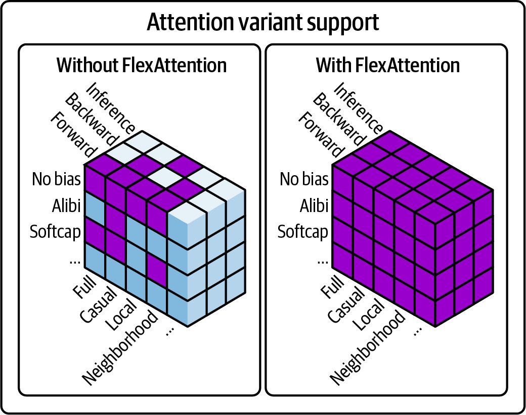
FlexAttention
    A compiler-based approach for custom sparsity patterns in attention. FlexAtten‐
    tion can be substantially faster for specific sparse attention patterns (e.g., block-
    sparse or sliding-window attention) by generating optimized kernels for these
    patterns, as shown in Figure 13-3. Use FlexAttention for special cases that
    scaled_dot_product_attention does not support.
PyTorch Optimized Attention Mechanisms | 553
Figure 13-3. FlexAttention provides support for custom attention variants
FlexDecoding
    This is a counterpart to FlexAttention that optimizes the decoding or text genera‐
    tion phases. FlexDecoding integrates with torch.compile and dynamic cache
    layouts. It uses compile-time optimizations for the decoder side of sequence gen‐
    eration, including KV caching efficiently across time steps. FlexDecoding can
    speed up autoregressive generation by reducing redundant compute during
    decoding. FlexDecoding is intended for LLM inference workloads, including
    those with long-generation sequences. It does not change training-time attention
    semantics.
Context parallel
   Context Parallel shards attention along the sequence-length dimension across
   participating devices or ranks to scale context length. Use the context_paral
   lel() API to scope replacement of scaled_dot_product_attention with
   context-parallel-aware kernels. The mechanism splits query-key-value (QKV) by
   sequence across ranks and synchronizes during attention, rather than paralleliz‐
   ing attention across threads within a single GPU.
554 | Chapter 13: Profiling, Tuning, and Scaling PyTorch
PyTorch Architecture Optimization (torchao), Quantization, Sparsity, and Pruning PyTorch Architecture Optimization (torchao) brings together quantization, sparsity, pruning, and related numerical-debugging tools into a single namespace. Its quanti‐ zation subpackage (torchao.quantization) provides common FX‐graph‐mode workflows, including post-training quantization (PTQ), quantization-aware training (QAT), and QConfigMapping APIs to convert and optimize models for INT8, FP8, and emerging formats. Beyond quantization, torchao supports pruning (torchao.pruning) and sparsity techniques like 2:4 and block sparsity (torchao.sparsity). These provide significant speedups with minimal loss in accuracy. torch.compile() integrates with the torchao framework for quantization. Under the hood, TorchDynamo captures each submodule’s computation as an optimized graph, then TorchInductor emits hardware-aware kernels that leverage torchao. This pro‐ duces consistent, end-to-end performance improvements for both model training and inference. Meanwhile, it preserves precise control over numerical formats and memory layouts. This makes it a great library for production-level performance opti‐ mizations such as quantization.
Concurrency with CUDA Streams As covered in an earlier chapter, CUDA streams enable concurrency and overlap of operations on the GPU. By default, PyTorch schedules all operations on the device’s default stream, stream 0, sequentially. However, many tasks are independent, and, if resources permit, a GPU can perform them in parallel using multiple streams. For example, GPUs can overlap data transfers with compute—or run separate neural net‐ work branches concurrently—by using separate, nondefault streams.
               Remember that modern GPUs have multiple DMA copy engines.
               Using separate streams for H2D copies can achieve truly parallel
               data transfers without blocking compute. This hardware support
               makes stream concurrency even more effective.
In PyTorch, you create a stream with torch.cuda .Stream(). You can then launch work on this stream using the Python context manager, with torch.cuda .stream(stream), or by explicitly assigning operations to that stream. PyTorch will issue operations (e.g., memory transfers, CUDA kernels, etc.) into the specified stream in a FIFO order—just as it does on the default stream.
Concurrency with CUDA Streams | 555
Overlapping Communication and Computation A common use of CUDA streams is to overlap host-to-device (H2D) data loading with GPU computation. This helps mask the data transfer latency incurred when using an external device such as a GPU—relative to the CPU running on the host. For instance, one stream can copy the next batch of input data from CPU to GPU memory while the default stream is busy training on the current batch. By the time the default stream is ready for the next batch, the data transfer is already done, and the GPU can process this next batch. This effectively hides the I/O latency. Here is an example of using two streams, the compute_stream (default) and the transfer_ stream (nondefault), to overlap data transfer and compute in PyTorch: # Set up streams device = 'cuda'
      # for H2D data transfers
      transfer_stream = torch.cuda.Stream(device=device)
      # for compute
      compute_stream        = torch.cuda.default_stream(device=device)
      # Create an iterator so we can preload "next" batches
      dataloader_iter = iter(dataloader)
      # Preload the very first batch onto GPU
      first_batch = next(dataloader_iter, None)
      if first_batch:
          with torch.cuda.stream(transfer_stream):
              next_inputs, next_labels = (
                  first_batch[0].to(device, non_blocking=True),
                  first_batch[1].to(device, non_blocking=True),
              )
      for _ in range(len(dataloader)):
          # 1) Wait for transfer of `next` batch to finish, then swap into compute var
          # Multiple copy engines allow H2D/peer copy concurrency.
          # Verify parallelism in Nsight Systems (Copy engines lanes)
          # And tracing/profiling tools (HTA, etc.)
          compute_stream.wait_stream(transfer_stream)
          inputs, labels = next_inputs, next_labels
           # 2) Kick off transfer of the *following* batch on the transfer_stream
           batch = next(dataloader_iter, None)
           if batch:
               with torch.cuda.stream(transfer_stream):
                   next_inputs, next_labels = (
                       batch[0].to(device, non_blocking=True),
                       batch[1].to(device, non_blocking=True),
                   )
556 | Chapter 13: Profiling, Tuning, and Scaling PyTorch
# 3) Run forward/backward on compute_stream with torch.cuda.stream(compute_stream): outputs = model(inputs) loss = loss_fn(outputs, labels) loss.backward() optimizer.step() optimizer.zero_grad(set_to_none=True) This example uses two CUDA streams: a dedicated transfer stream for asynchronous host-to-device copies and the default compute stream for model work. This hides H2D latency and matches PyTorch’s recommended pattern for overlapping commu‐ nication and computation. Specifically, while the model is processing a batch on the default stream, the next batch’s data transfer is already underway on the transfer_stream. Synchronizing with compute_stream.wait_stream(transfer_stream) before consuming the pre‐ loaded batch enforces correct ordering without a full device-wide barrier. And the .to(device, non_blocking=True) calls make sure that the copy uses asynchro‐ nous DMA-based copies that don’t block the calling CPU thread. Using next(dataloader_iter, None) gives explicit control over when transfers are enqueued versus when the kernel operations run. This makes sure one batch of data is moving on the transfer stream while another batch is executing on the compute stream, as shown in Figure 13-4.
Figure 13-4. Overlapping compute and data transfer with dedicated compute and transfer streams
Additionally, by pulling from dataloader_iter ahead of time and storing in next_inputs next_labels, this code separates batch loading (running on the CPU in transfer_stream) from batch processing (running on the GPU in compute_stream).
Concurrency with CUDA Streams | 557
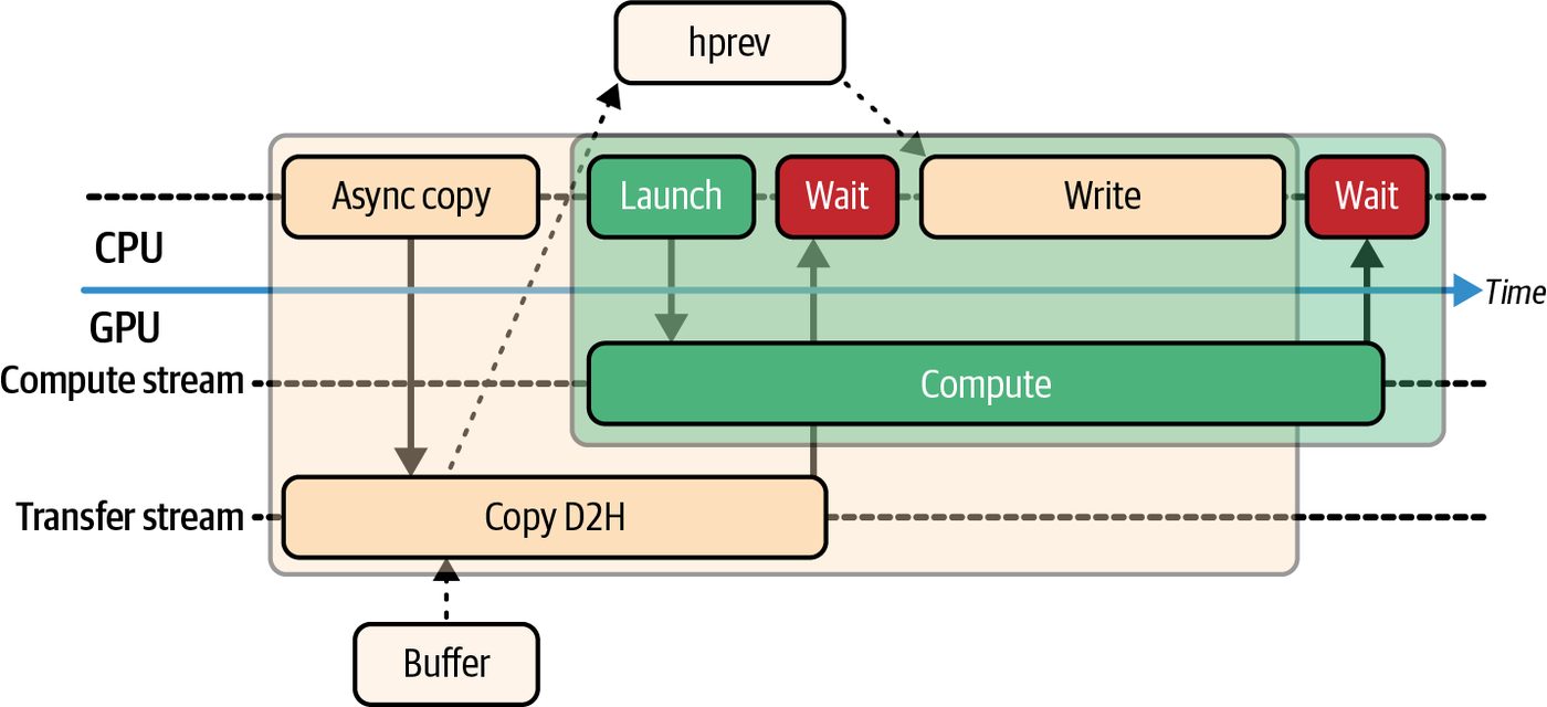
This split means you always have one batch in flight for each stream. This decouples data loading from compute and maximizes overlap.
                     Always profile with Nsight Systems or the PyTorch profiler when
                     adding streams. Look at GPU utilization, and, if done correctly,
                     you’ll see near 100% utilization with transfer and compute overlap‐
                     ping. If utilization drops—or you see data transfers and compute
                     happening sequentially—double-check for any implicit synchroni‐
                     zations such as CUDA tensor print()—or extra CUDA
                     synchronizations in your code.
Stream Synchronization with Events When using multiple streams, it’s sometimes necessary to coordinate between them to make sure that one stream’s work is done before another stream uses its results, for instance. A lightweight way to synchronize specific points is using CUDA events, as discussed in Chapter 11. With CUDA events, you can record an event on one stream and make another stream wait for that event. This avoids the heavyweight full synchronization of torch.cuda.synchronize() and, instead, synchronizes only the necessary streams needed to process an individual event. In fact, even in a multi-GPU context, events can be used to synchronize work across devices. In this case, one GPU records an event on its device stream while another GPU waits for the event on its device stream. This is how NCCL handles dependen‐ cies under the hood. By using events smartly, you keep the multiple GPUs working in parallel as much as possible. Next is an example of using CUDA events to synchronize two streams, stream1 and stream2 in PyTorch: # Disable timing on the event since we’re using it purely for synchronization. event = torch.cuda.Event(enable_timing=False)
      # In first stream:
      with torch.cuda.stream(stream1):
          kernel_launch(...)
          event.record()           # record event at end of work in stream1
      # In another stream or on host:
      stream2.wait_event(event)    # make stream2 wait until event is signaled
      with torch.cuda.stream(stream2):
          other_kernel_launch(...)
In this code, we record an event at the end of some work on stream1. Later, before launching work on stream2, we call stream2.wait_event(event). This inserts a
558 | Chapter 13: Profiling, Tuning, and Scaling PyTorch
dependency such that stream2 will not execute its next kernel until the event is sig‐ naled by stream1 reaching that point. Events are useful for scheduling lightweight dependencies between streams, as they avoid heavy, global synchronizations that will stall all stream execution. Let’s revisit the PyTorch data loader/overlap example in the previous section and rewrite it to synchronize with CUDA events. We are using the same pair of streams from earlier (transfer_stream and compute_stream), but we’re adding a transfer_ done CUDA event to synchronize at a fine-grained, event-specific level: import torch
device = 'cuda'
    # for H2D copies
    transfer_stream = torch.cuda.Stream(device=device)
    # for compute
    compute_stream = torch.cuda.default_stream(device=device)
    # sync-only event (low overhead)
    transfer_done = torch.cuda.Event(enable_timing=False)
    # Iterator so we can preload ahead
    dataloader_iter = iter(dataloader)
    # ---- Preload first batch ----
    first_batch = next(dataloader_iter, None)
    if first_batch:
        with torch.cuda.stream(transfer_stream):
            next_inputs, next_labels = (
                first_batch[0].to(device, non_blocking=True),
                first_batch[1].to(device, non_blocking=True),
            )
            # mark when H2D is done
            transfer_done.record(stream=transfer_stream)
    for _ in range(len(dataloader)):
        # ---- Sync: wait for the transfer to complete ----
        compute_stream.wait_event(transfer_done)
        inputs, labels = next_inputs, next_labels
        # ---- Kick off next transfer ----
        batch = next(dataloader_iter, None)
        if batch:
            with torch.cuda.stream(transfer_stream):
                next_inputs, next_labels = (
                    batch[0].to(device, non_blocking=True),
                    batch[1].to(device, non_blocking=True),
                )
                transfer_done.record(stream=transfer_stream)
Concurrency with CUDA Streams | 559
# ---- Compute on the compute stream ---- with torch.cuda.stream(compute_stream): outputs = model(inputs) loss = loss_fn(outputs, labels) loss.backward() optimizer.step() optimizer.zero_grad(set_to_none=True) This is the same overlap pattern as the previous section, but it uses a CUDA event for the transfer → compute synchronization. This is in contrast to the wait_stream() mechanism used in the other example. This code still uses next(dataloader_iter) to preload batches ahead of time (same as the example in the previous section). This way, data transfer and compute are always overlapping. However, in this example, the transfer_done event is recorded with trans fer_done.record(stream=transfer_stream) on the transfer_stream right after the asynchronous copy is enqueued. This timestamps the event. The compute_stream.wait_event(transfer_done) then stalls the compute_stream until the copy is complete and the transfer_done event is triggered. It then consumes the prefetched batch and performs its compute operations on the compute_stream. Besides data loading, CUDA streams are useful in a lot of different contexts. Let’s dis‐ cuss how they’re used in MoE models.
Using CUDA Streams with MoE Models In practice, transformer-model layers are sequentially dependent, so you can’t arbi‐ trarily run layers in parallel. However, in an MoE architecture, different experts can run concurrently on separate CUDA streams since their computations are independent. Each expert processes a distinct segment of the input. At the join point, the expert outputs are aggregated. It’s essential that each expert writes only to its assigned slice of the output tensor. If two experts accidentally write to overlapping memory regions, this will introduce a race condition, which can corrupt the results—or trigger syn‐ chronization issues caused by the nondeterministic order of writes from the experts. To avoid such issues, you should make sure to use proper stream-level synchroniza‐ tion (e.g., stream events) and verify that memory is cleanly partitioned across expert kernels. By enforcing this separation between expert execution and output aggrega‐ tion, you will maintain correctness without sacrificing parallelism.
560 | Chapter 13: Profiling, Tuning, and Scaling PyTorch
               NVIDIA’s Compute Sanitizer can detect concurrency and synchro‐
               nization issues in CUDA code, including race conditions and dead‐
               locks. Also, you can set CUDA_LAUNCH_BLOCKING=1 to force
               synchronous kernel execution. This will surface ordering and
               dependency bugs by making kernel execution deterministic. This
               will reveal if outputs are being consumed before they’re fully
               produced.
In our example, each expert could, in theory, run on its own stream—or even its own GPU if the framework is extended to multiple GPUs. In this case, synchronization— ideally using stream events—is needed when gathering the results. Pipeline parallelism, or pipelining microbatches through different model stages on different devices, and serving multiple inference requests are two scenarios that natu‐ rally benefit from multiple streams. In a pipeline parallel workflow, for instance, each stage of the model has its own stream that processes a different microbatch concur‐ rently. Meanwhile, it’s also communicating with neighboring stages. In multirequest inference serving, each request’s model execution can be launched in its own stream. With sufficient hardware resources, this can increase throughput by overlapping inference computations—at the cost of some per-request latency due to resource-sharing overhead. In short, CUDA streams help to squeeze extra performance out of your hardware by overlapping work across multiple kernels, stages, or requests. They require careful synchronization to avoid race conditions. But, when used correctly, they can hide latency and keep a GPU more fully utilized. It’s recommended to continuously profile your code when introducing concurrency. And keep in mind that sequential execution at 100% utilization may actually perform better than parallel execution that introduces resource contention. Often, though, streams let you utilize parts of the GPU that would otherwise sit idle. Finding the right balance is important.
               Always make sure you are launching on the intended stream. Acci‐
               dentally using the default stream, for example, can reintroduce
               unnecessary serialization. This is easy to mess up, so it’s worth
               repeating again.
Concurrency with CUDA Streams | 561
Reducing Kernel Launch Overhead with CUDA Graphs We’ve seen in earlier chapters that CUDA Graphs eliminate per-iteration launch over‐ head, reduce CPU launch overhead, and eliminate tiny idle gaps between kernels. And removing even the smallest idle gaps leads to higher effective utilization—and more consistent iteration times. Now let’s show how to use them in PyTorch.
Capturing a CUDA Graph and Preallocating Memory PyTorch provides a torch.cuda.CUDAGraph API to capture and replay CUDA Graphs. The general usage pattern is to first warm up the model by running a few iterations normally to initialize all necessary data and allocations. Next, you create a CUDAGraph object and a dedicated, nondefault CUDA stream to isolate the capture.
                     When using "reduce-overhead" or "max-autotune", the compiler
                     will automatically capture CUDA Graphs for you if the model is
                     stable. In this case, you don’t even need to write this boilerplate
                     since it’s done for you automatically if you’re using the PyTorch
                     compiler with these modes. And if your model has varying shapes
                     each iteration, consider the "max-autotune-no-cudagraphs" mode
                     to avoid graph capture, as CUDA Graphs currently require static
                     shapes.
You then perform a full pass of the model’s execution to record the sequence of oper‐ ations using the capture stream specified in the torch.cuda.graph() context. Once the operations are captured in the CUDA Graph, you can replay() the graph on new inputs as needed (e.g., model training or inference.) Before capturing a CUDA Graph, all static memory used during capture must be preallo‐ cated—and preferably at its maximum size. These buffers include inputs, outputs, and intermediate tensors. If any new memory allocation happens during capture, the graph will fail with an error such as “operation not permitted when stream is capturing.” To reduce fragmentation and maximize contiguous memory space for these fixed buffers, you can invoke torch.cuda.empty_cache() immediately before entering the capture block. This will clear unused cached memory and give the allocator the best chance to lay out your prereserved buffers without interruption.
                     Frequent use of torch.cuda.empty_cache() can disrupt allocator
                     efficiency and incur longer-term performance costs. Treat this call
                     as a one-time safety mechanism when capturing a graph—and not
                     a regular maintenance tool.
562 | Chapter 13: Profiling, Tuning, and Scaling PyTorch
Remember that PyTorch’s caching allocator supports CUDA’s asynchronous allocator (cudaMallocAsync) to reuse fixed memory addresses. However, this does not bypass CUDA Graphs’ requirement to not create new allocations within the graph. You still need to allocate fixed-size buffers upfront to avoid a runtime error if you try to allocate new memory inside the graph. Make sure all tensors reach their maximum required size during the warm-up prior to graph capture. We’ll cover more about this in the upcoming graph replay section. You need to use a dedicated, nondefault stream for graph capture to avoid interfer‐ ence with any operations that should not be included in the CUDA Graph. Here is a code snippet demonstrating how to capture a CUDA Graph in PyTorch with a dedi‐ cated capture_stream: g = torch.cuda.CUDAGraph() capture_stream = torch.cuda.Stream()
    # Prepare static inputs and outputs
    static_input = torch.randn(batch_shape, device='cuda')
    static_output = torch.empty(output_shape, device='cuda')
    # Warm-up step on capture_stream to allocate buffers without recording
    with torch.cuda.stream(capture_stream):
        tmp = model(static_input)
        static_output.copy_(tmp)
    # ensure warm-up is complete
    capture_stream.synchronize()
    # Begin graph capture
    with torch.cuda.graph(g, stream=capture_stream):
        tmp = model(static_input)
        static_output.copy_(tmp)
    # ensure capture is complete before using the graph
    capture_stream.synchronize()
In this code, we first allocate static_input and static_output on the GPU with fixed shapes. We run one warm-up iteration on capture_stream to ensure that any memory needed inside model(static_input) is allocated—and to perform any onetime setup.
                By preallocating the output buffer and using static_out
                put.copy_(tmp) in both warm-up and capture phases, the code
                writes its results into a fixed memory region. This makes the cap‐
                tured CUDA Graph correct, replayable, and reproducible without
                unexpected tensor allocations.
Reducing Kernel Launch Overhead with CUDA Graphs | 563
We then synchronize the capture_stream to make sure that the warm-up step is fully complete before beginning the actual graph capture. Next, we enter the torch.cuda.graph(...) context on the same stream and rerun the model forward pass. During the capture phase, no kernels are actually launched. Instead, the operations are just recorded into the CUDA Graph object g. After exiting the capture block, we need to synchronize once more to make sure the recording is finalized. When capturing a CUDA Graph, strict isolation is essential. Operations on the cap‐ ture stream must not be affected by activity on any other streams. Even a seemingly unrelated kernel launch on another thread can invalidate the capture. This could lead to runtime errors like “operation not permitted when stream is capturing.” This error happens if you accidentally perform CUDA operations on other streams while the capture is in progress. In this case, it invalidates the graph context and trig‐ gers this error. This can also happen if you launch a kernel on the capture stream that performs dynamic memory allocation, like tensor creation or calling torch.empty during capture.
                     Always call capture_stream.synchronize() both before starting
                     the graph capture and after exiting it. This ensures that all opera‐
                     tions are correctly recorded and that the graph is ready for safe
                     replay. The previous code example follows this best practice.
After capturing the graph, it can be replayed on any stream, including the default stream—and regardless of which stream was used for capture. If you trigger any CUDA operations that depend on the graph completing fully, you must synchronize before running the operations, as shown next. Otherwise, because the graph runs asynchronously when replayed, the CUDA operations that depend on the graph results may run before the graph completes execution: # replay the graph which writes to static_output g.replay()
      # synchronize on the stream that is replaying the graph
      torch.cuda.current_stream().synchronize()
      # Now it's safe to read or post-process the output
      print(static_output)
564 | Chapter 13: Profiling, Tuning, and Scaling PyTorch
Without this explicit synchronization, your program could proceed and incorrectly assume that the graph has finished executing and written its results to static_out put. If no synchronization is in place, the code may read stale or partially written data because the graph may not have finished writing to static_output. This scenario will cause nondeterministic behaviors, corrupted reads, subtle race conditions, and deadlocks.
Replaying the Graph To replay the graph with new data, you copy the new inputs into the preallocated input tensors, static_input, and call g.replay(). The GPU will execute the entire captured sequence of operations using the current contents of those tensors as input. The graph will place the results in the preallocated output tensor (static_output), as shown here: # load new data into pre-allocated input tensor static_input.copy_(new_batch)
    # execute the captured graph
    g.replay()
    # retrieve the output (clone if you plan to modify it)
    result = static_output.clone()
Here, we load new_batch data into the memory space of static_input and then call g.replay(). The graph runs the exact captured operations using the current static_input data and writes the outputs into static_output. We can then use or clone static_output as needed. It’s recommended to validate that the graph’s output matches a normal execution for a few test inputs to make sure the capture was successful. Also, remember that you can‐ not directly print or call .item() on static_output without syncing. If needed, do result = static_output.cpu().numpy() after replay and outside of any asynchro‐ nous regions for debugging. Since the graph reuses the same input, output, and internal memory allocations each time, it will overwrite the same output tensor on each iteration. So if you need to pre‐ serve the output beyond a single iteration, you need to clone() the buffer, as shown in the previous code. This is why we need to make sure that the allocations in the warm-up/capture step cover the maximum sizes needed. Remember that the graph cannot handle additional memory allocations on the fly.
Reducing Kernel Launch Overhead with CUDA Graphs | 565
It’s worth noting that after using a CUDA Graph, certain PyTorch operations will not be reflected until you recapture the graph. For instance, if you change model weights on the fly and outside of the graph, these updates won’t apply because the graph has its own copy of operations. As such, graphs work best in steady-state loops in which operations are repeated on each iteration. Also, when using cudaMallocAsync to preallocate memory for a CUDA Graph, it will reuse the same memory addresses during replay that it preallocated during graph capture—or during warm-up if the graph is loaded from disk, for instance. This way, subsequent graph replays do not require additional memory. By default, every instance of a CUDA Graph uses its own private memory pool. This way, you’re guaranteed that each graph preallocates its own memory buffers and does not compete with other instances of the graph. In other words, two identical graphs will not compete for memory if they’re replayed concurrently since they each use their own memory pool and buffer space. You can choose to share a memory pool between graph instances by passing torch.cuda.graph(pool=...). However, this is useful only in very special cases when you want to purposely orchestrate related graphs to reuse the preallocated memory buffers for performance reasons. For example, consider simultaneously run‐ ning multiple inference graph variants—each using a different batch size (e.g., 1, 2, 4, 8, etc.). In this case, you can reduce overall memory usage by having the shapespecialized variants reuse a single, large memory allocation for PagedAttention, which uses a varying-size tensor called block_tables. This approach is described in a FireworksAI blog post. Here, they compile a different CUDA Graph variant for each batch size. And, instead of creating a separate memory pool for each graph, they share a single shared memory pool across all graph variants. By compiling graphs in decreasing order of batch size, memory from the shared pool is reused from the largest variant (e.g., 8, in this case). Smaller batch-size graph var‐ iants are serviced by the larger allocated buffers from a previous iteration. This way, multiple graph variants are supported without using excessive GPU memory.
                     This is an obscure and clever implementation choice that requires
                     careful coordination of the memory segments. However, it does
                     reduce the total GPU memory usage when running multiple shape-
                     specialized graphs simultaneously. This is great for deployment sce‐
                     narios in which minimizing overall memory usage is critical.
566 | Chapter 13: Profiling, Tuning, and Scaling PyTorch
Best Practices for CUDA Graphs
CUDA Graphs are a powerful way to reach peak steady-state throughput in both
training and inference. They are especially useful for large deployments in which
CPU overhead and kernel-launch variability are hurting performance. On modern
GPUs, which execute thousands of operations extremely quickly, graphs become
essential to keep the GPU devices busy and minimize per-kernel launch overhead.
It’s worth noting that PyTorch’s torch.compile uses CUDA Graphs under the hood
in many cases—unless explicitly disabled. CUDA Graphs are used to minimize kernel
launch overhead for compiled models. Here are a few important things to remember
when using CUDA Graphs:
Avoid allocating memory during graph capture
    Remember that you can’t dynamically allocate GPU memory inside the graph
    capture. Any tensor that’s needed should be allocated beforehand during the
    warm-up step, as shown previously. If your graph needs temporary buffers, use
    PyTorch’s graph-aware caching allocator using the cudaMallocAsync CUDA
    backend. This way, each replay reuses the same buffer addresses. Make sure these
    temporary tensors are created during the warm-up phase (before graph capture)
    using their maximum potential size. This will preallocate all the needed memory
    upfront.
Keep the graph structure fixed
    A captured graph cannot change the sequence of operations, tensor shapes, or
    memory sizes. If your workload has occasional shape variations, one strategy is
    to capture multiple graphs (e.g., one for each input size you expect) and then
    select the appropriate graph at runtime. Alternatively, you can disable graphs for
    those iterations (PyTorch’s compiler has a mode max-autotune-no-cudagraphs
    for such cases).
                   CUDA supports a low-level Graph Management API, includ‐
                   ing cudaGraphExecUpdate(), described in an earlier chapter,
                   which allows minor modifications to a captured graph. How‐
                   ever, as of this writing, PyTorch does not expose this. Within
                   PyTorch currently, it’s best to treat graphs as immutable.
Capture as much as possible Include as much of the training loop as you can in the graph—ideally an entire iteration (forward pass, backward pass, optimizer step, and any all-reduce com‐ munications). The more you capture, the more CPU overhead and launch latency you eliminate.
Reducing Kernel Launch Overhead with CUDA Graphs | 567
      Also, consider capturing multiple iterations in one graph if memory allows
      (including loop unrolling, etc.). Although this makes the graph bigger, it can
      often improve throughput by enabling even more optimizations across iterations.
      This comes at the cost of flexibility, but it’s worth exploring and profiling.
      When capturing large graphs in multi-GPU setups, use CUDA stream priorities
      if supported. For instance, you can set NCCL calls to a lower-priority stream if
      you want the compute kernels to run at a higher priority and not be delayed.
      Graph capture will record these priorities as well.
                           NVIDIA’s MLPerf submissions (and internal benchmarks)
                           often capture the entire training step into one graph per itera‐
                           tion. This includes the forward pass, backward pass, optimizer,
                           and all-reduce communication steps. This eliminates nearly all
                           runtime overhead (launch jitter, etc.), at the expense of mem‐
                           ory and flexibility.
Plan for memory reuse
    After a graph is captured, you can’t free or reallocate any tensors used by that
    graph—or change any of their sizes. It’s best to reserve a bit more capacity than
    needed by capturing with the maximum batch size that you expect. This way, a
    slightly larger input won’t break the graph later during replay.
      For example, if your maximum batch size is 64 but you occasionally run with 96,
      consider capturing with batch size 96 just to be safe. It’s usually better to capture
      the worst-case scenario, run smaller batches, and waste a bit of memory—rather
      than risking a graph failure.
                     Remember to account for the sizes of the optimizer states (e.g., the
                     Adam optimizer intermediate buffers) since they’re part of model-
                     training graphs. These are somewhat easy to forget!
When used appropriately, CUDA Graphs can provide significant speedups for large model training and inference workloads. With compute optimizations in place, let’s turn to memory optimizations in PyTorch.
CUDA Graph Trees (PyTorch Compiler Internal) We’ve covered the PyTorch compiler in a previous section, but in the context of CUDA Graphs, it’s worth mentioning PyTorch’s CUDA Graph Trees. These are used by torch.compile, and specifically mode="reduce-overhead", to compile and cache separate static graphs for each input shape.
568 | Chapter 13: Profiling, Tuning, and Scaling PyTorch
Once a static graph is recorded, its tensor dimensions must remain fixed. Any new input shape will trigger a fresh recording and cache entry. To maximize cache hits and reduce graph captures, it’s recommended to keep your input shapes as consistent as possible across iterations. Fewer distinct shapes mean more reuse of the recorded graphs and less overhead. It’s worth noting that you don’t typically invoke the CUDA Graph Trees API directly. This is handled for you by torch.compile when specifying mode="reduceoverhead". Since CUDA Graphs require static addresses and steady control flow, full-graph cap‐ ture is difficult for LLM inference, which supports variable input sizes, batch sizes and number of steps (e.g., sampling, KV cache growth, host-side decisions, etc.) For model training, CUDA Graph Trees allow multiple captured subgraphs to share a single memory pool across forward and backward captures. CUDA Graph Trees are also useful for inference since they allow dynamic subgraph selection depending on the input shape and batch size. This is commonly called “piecewise capture.” PyTorch leverages CUDA Graph Trees to maintain per-shape piecewise captures and manage shared pools.
               The piecewise capture pattern provided by CUDA Graph Trees is
               the mechanism used by the vLLM inference engine to support dif‐
               ferent graphs for different input shape and batch-size combina‐
               tions. We cover vLLM and inference-engine optimizations in more
               detail starting in Chapter 15.
Profiling and Tuning Memory in PyTorch Large models can be limited by GPU memory capacity and memory bandwidth. Additionally, inefficient memory use such as memory fragmentation can hurt perfor‐ mance even if HBM capacity is sufficient. You can address memory issues on several fronts, including memory-allocator tuning, activation checkpointing, memory off‐ loading, and input-pipeline optimization. Also, PyTorch has a memory profiler that’s built into torch.profiler by enabling profile_memory=True, as shown earlier. You can use this to find out which opera‐ tions allocate a lot of memory—and try to address those operations first, as shown in the visualization in Figure 13-5 generated by the PyTorch memory visualizer tool.
Profiling and Tuning Memory in PyTorch | 569
Figure 13-5. PyTorch memory profile visualization for three iterations of a forward and backward pass
Also, NVIDIA’s Nsight System’s CUDA Memory Inspector can help visualize how memory fragmentation happens over time. Utilizing these can guide your memoryallocator tuning efforts, as we’ll explore next.
Tuning the CUDA Memory Allocator PyTorch uses a caching memory allocator for CUDA memory. By default, it adapts to allocation patterns by splitting and recycling GPU memory blocks on demand. How‐ ever, certain workload patterns that use variable-sized memory allocations can lead to memory fragmentation. Memory fragmentation happens when GPU memory gets split into many noncontig‐ uous free chunks over time. This makes it difficult to allocate a large tensor even if enough total memory remains free. In MoE models, this is especially problematic because the number of tokens routed to each expert can change with every batch. As such, each expert’s output activation tensor may be a different size on every iteration. Variable-sized memory allocations leave behind uneven, fragmented memory blocks. These fragment memory blocks accumulate across training or inference runs. To avoid this, you should allocate a fixed-size expert output buffer upfront and size it to the maximum possible number of tokens any expert may process in your batch. Then you can reuse this buffer on every iteration. By keeping the buffer dimensions constant, the GPU memory allocator won’t frag‐ ment memory over time. Each expert writes into its slice of the preallocated buffer rather than triggering new allocations. This method stabilizes memory usage, improves reuse efficiency, and avoids fragmentation-related failures or slowdowns.
570 | Chapter 13: Profiling, Tuning, and Scaling PyTorch
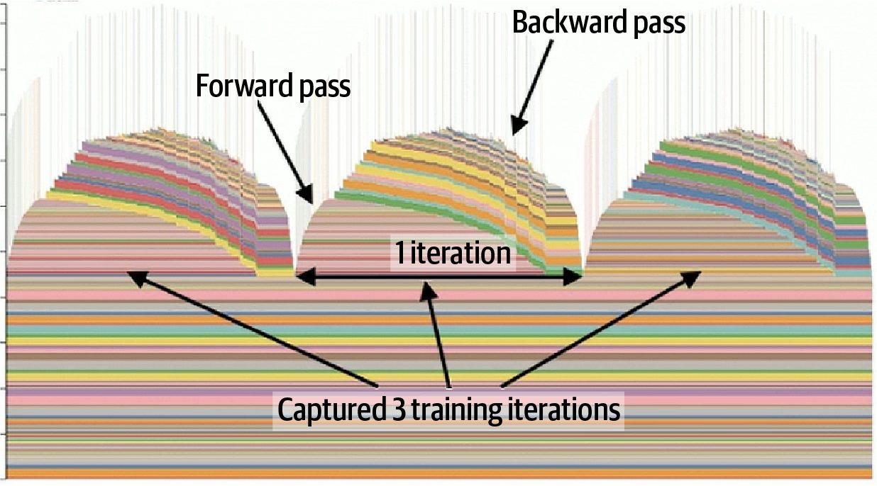
You can adjust PyTorch’s allocator configuration using an environment variable to
tune its behavior. Here is an example:
    export PYTORCH_ALLOC_CONF=\
    max_split_size_mb:256,\
    roundup_power2_divisions:[256:1,512:2,1024:4,>:8],\
    backend:cudaMallocAsync
Next is a description of each specified configuration parameter in the code:
max_split_size_mb:256
    This parameter instructs the allocator to keep large free blocks intact (up to 256
    MB) rather than continually splitting them into tiny pieces. This helps reduce
    fragmentation. By default, PyTorch splits large allocations less aggressively. Set‐
    ting max_split_size_mb explicitly allows large contiguous free blocks to be avail‐
    able for large neural network layers in modern LLMs.
roundup_power2_divisions:[N:M,...]
    This parameter controls how PyTorch’s CUDA caching allocator groups requests
    for tensor sizes into fixed buckets. It divides each “power-of-two” range into N
    equal subbuckets—for example, if a request falls between 512 MB and 1,024 MB.
    With 512:2 specified in the code, the range between 512 and 1,024 MB is divided
    into :2 buckets and rounded up to one of [512MB, 768 MB, 1 GB]. For example,
    in the 512 to 1,024 MB range with '512:2', a 600 MB request rounds up to 768
    MB. Check allocator logs to confirm actual bucketing in your environment. This
    strategy reduces memory fragmentation, standardizes allocation sizes, and
    increases cache reuse since similar requests hit the same bucket.
backend:cudaMallocAsync
    Specifying this will enable NVIDIA’s CUDA asynchronous allocator as the under‐
    lying memory-allocation mechanism. This can help avoid synchronizations on
    memory free events—and can improve performance in multithreaded contexts
    like multiworker data loading.
By customizing a memory allocator configuration, you can maintain a steadier, more
predictable memory usage pattern. You can monitor memory fragmentation with
torch.cuda.memory_stats() over long runs to make sure your memory footprint
stays stable and doesn’t explode in size.
You can also use torch.cuda.mem_get_info() at runtime to get free versus total
memory. This tracks fragmentation indirectly since, if free memory drops while the
number of allocated tensors stays constant, fragmentation is increasing.
Profiling and Tuning Memory in PyTorch | 571
Activation Checkpointing for Memory Savings For extremely large models, activation checkpointing, also called gradient check‐ pointing by some practitioners, is essential to manage memory. With a large LLM, it’s sometimes not possible to store all intermediate activations for backpropagation without running out of memory. With activation checkpointing, instead of storing intermediate activations during the forward pass (to be used on the backward pass), you can recompute them on the fly during the backward pass only when needed. PyTorch provides torch.utils.check point to automate this. You simply wrap your model layer—or sequence of layers— and their forward activations won’t be stored. You can apply checkpointing at the granularity of each transformer block and each expert Feedforward Neural Network (FFN) layer in your mode. This way, after com‐ puting each block’s forward output, you don’t need to keep those intermediate activa‐ tions in memory. Instead, during the backward pass, PyTorch will rerun that block’s forward pass to regenerate the activations for gradient computation. It’s worth noting that you don’t have to checkpoint everything. You can just focus on the largest layers. A common strategy is checkpointing only the transformer blocks, which hold a massive number of activations, but not checkpointing the smaller layers like layer norms and embedding layers. This produces the most memory savings with minimal recompute overhead.
                     When using FSDP, you can also enable automated checkpointing,
                     which will recursively apply checkpointing to multiple layers for
                     you.
This trade increases compute for reduced memory usage. Fortunately, modern GPUs provide abundant FLOPS relative to the amount of HBM memory, so this technique is a natural fit for the latest generations of hardware. As such, the GPU has extra compute headroom to afford these extra recomputations. This trade-off often proves worthwhile. Without activation checkpointing, you would need to reduce your input batch size—or the number of experts—to fit into limited GPU memory. With checkpointing, however, you can comfortably fit the model into memory and preserve the larger batch size. And while activation checkpointing slows training down a bit, it allows you to train larger model variants—and use larger input batch sizes—that would otherwise not fit into memory. Essentially, you exchange some of the GPU’s ample compute FLOPS to overcome its limited HBM capacity.
572 | Chapter 13: Profiling, Tuning, and Scaling PyTorch
Offloading Parameters to CPU and NVMe In addition to checkpointing, you can offload some of the models’ parameters that don’t need to be actively stored on the GPU. For instance, an MoE model has some less frequently accessed expert layers that could be offloaded to CPU memory—and transfer them to the GPU only when needed. It’s important to overlap transfers with computations such that while one layer is run‐ ning on GPU, it’s asynchronously prefetching the next layer’s weights from CPU or SSD. In practice, frameworks like DeepSpeed’s ZeRO-Infinity (for training) and ZeRO-Inference (for inference) can automate this prefetching. They stream model weights layer-by-layer from CPU or NVMe to GPU, minimizing peak GPU memory usage while overlapping data transfers with computation. You can pin these components on the host and use asynchronous, nonblocking DMA calls like .to(device) and cudaMemcpyAsync to transfer them into the GPU while other computations are running. This will hide the extra transfer latency incurred by copying from the CPU. NVIDIA’s Unified Memory is also an option—especially for superchip systems like Grace Blackwell GB200/GB300 with high-speed interconnects like NVLink-C2C between the CPU and GPU. In these cases, Unified Memory allows rarely used GPU memory pages to be evicted to the CPU’s system memory. The OS may even swap them to NVMe/SSD if needed for capacity. NVMe should be used as a last resort through normal OS swapping, not as a primary target of Unified Memory. However, unified memory can introduce unpredictability due to memory paging, etc. As such, explicitly managing the offloading is often preferable to maintain full con‐ trol and predictable performance. Recent advancements like GPUDirect Storage allow GPUs to directly read from NVMe drives. This means that, in some cases, your model parameters could be paged directly from NVMe on the fly without any CPU involvement. This is useful for both training and inference serving when using massive models. For larger models on the order of trillions of parameters, you can offload components to NVMe storage and swap them into GPU memory just-in-time. The key is to over‐ lap the data transfers with computations so they don’t stall the training loop.
SuperOffload: Optimized CPU-GPU Superchip Offload SuperOffload is an offload system designed specifically to take advantage of CPUGPU superchip hardware efficiencies. Superchips (e.g., Grace Hopper, Grace Black‐ well, Vera Rubin, etc.) provide high-bandwidth NVLink-C2C interconnects between the CPU and GPU. Combined with a shared, coherent memory address space, a
Profiling and Tuning Memory in PyTorch | 573
superchip-optimized offload strategy can produce huge speedups and utilization gains compared to traditional offload techniques. There are a few key innovations that SuperOffload demonstrates including speculation-then-validation (STV), heterogeneous optimization computations, superchip-aware data type conversions, and memory copies. Let’s discuss each of these next. Compared to traditional offloading, which waits for gradient reduction and global checks before updating parameters, STV overlaps these steps by performing specula‐ tive optimizer updates on the CPU while backpropagation is running on the GPU. It then validates the results afterward. This effectively reduces synchronization stalls and improves overall GPU utilization. SuperOffload uses heterogeneous optimizer computations to partition optimizer work between the CPU and GPU. For instance, it assigns compute-heavy tensors updates to the GPU while CPU cores handle lighter state updates such as momentum buffers used by the Adam optimizer. This keeps both devices busy, reduces idle cycles, and increases overall chip utilization. Because NVLink-C2C provides high bandwidth between the CPU and GPU, Super‐ Offload can change the precision and placement strategy for tensor type casts and data transfers. By shifting type conversions and copies toward the GPU, SuperOffload takes advantage of the fast, coherent interconnects to minimize CPU-GPU transfer latency. In addition, SuperOffload uses a CPU-optimized variant of the Adam optimizer called GraceAdam, which is designed for Grace’s ARM Scalable Vector Extension (SVE) architecture. SVE is a long-vector architecture used by the ARM A64 instruc‐ tion set. Specifically, it has 32 vector registers and 16 predicate registers that, in com‐ bination with SuperOffload, help to improve throughput and energy efficiency for offloaded parameter updates.
FSDP Automatic Checkpointing and Offloading PyTorch’s FSDP is a distributed parallelism strategy that shards model parameters, gradients, and activations across GPUs during model training. This reduces memory overhead during training—and lets you train larger models than you could without sharding. Technically, FSDP implements the ZeRO Stage-3 strategy to shard model states across GPUs, as shown in Figure 13-6.
574 | Chapter 13: Profiling, Tuning, and Scaling PyTorch
Figure 13-6. FSDP shards model parameters, gradients, and optimizer states across the GPUs (ZeRO Stage-3)
FSDP can automatically apply activation checkpointing and offload parameters/
gradients under the hood. Simply wrap the model with FSDP(), then specify the
activation_checkpointing_policy and CPUOffload parameters as shown here:
    import torch
    import torch.nn as nn
    import torch.distributed as dist
    from torch.distributed.fsdp import (
Profiling and Tuning Memory in PyTorch | 575
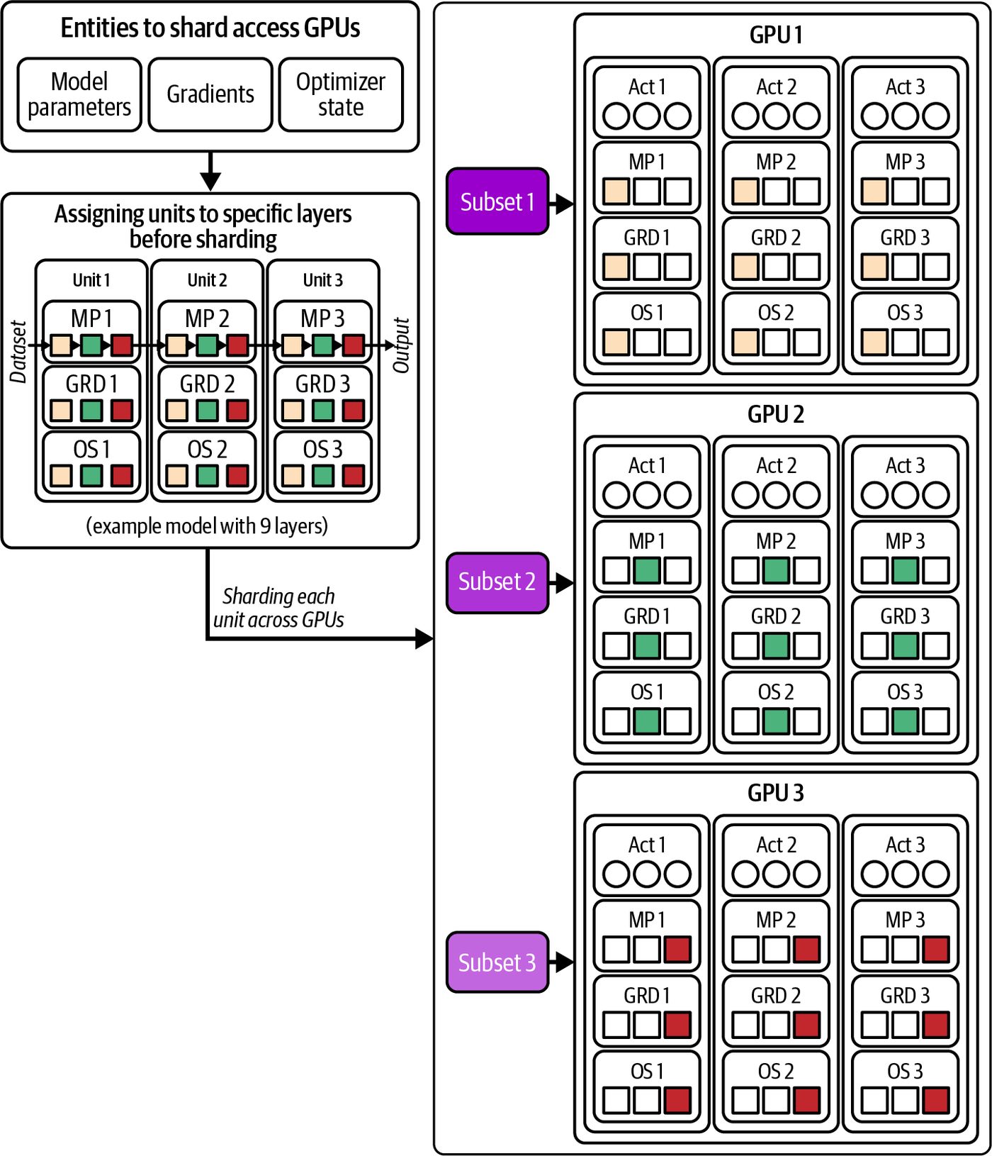
             FullyShardedDataParallel as FSDP,
             CPUOffload, ShardingStrategy, BackwardPrefetch, MixedPrecision
      )
      from torch.distributed.fsdp.wrap import transformer_auto_wrap_policy
      # Initialize distributed
      dist.init_process_group("nccl")
      torch.cuda.set_device(dist.get_rank() % torch.cuda.device_count())
      # Build your model
      class MyModel(nn.Module):
          def __init__(self):
              super().__init__()
              self.layers = nn.Sequential(
                  nn.Linear(4096, 4096),
                  nn.ReLU(),
                  nn.Linear(4096, 4096),
              )
             def forward(self, x):
                 return self.layers(x)
model = MyModel().cuda()
      # Auto-wrap transformer blocks if needed
      auto_wrap_policy = transformer_auto_wrap_policy(
          model,
          min_num_params=1e8,
      )
      # Wrap with FSDP + checkpointing + CPU offload
      fsdp_model = FSDP(
          model,
          auto_wrap_policy=auto_wrap_policy,
          sharding_strategy=ShardingStrategy.FULL_SHARD,
          use_orig_params=True,
          cpu_offload=CPUOffload(offload_params=True, pin_memory=True),
          mixed_precision=MixedPrecision(
              param_dtype=torch.bfloat16,
              reduce_dtype=torch.bfloat16,
              buffer_dtype=torch.bfloat16
          ),
          backward_prefetch=BackwardPrefetch.BACKWARD_PRE,
          activation_checkpointing_policy={
              nn.TransformerEncoderLayer,
              nn.TransformerDecoderLayer,
              nn.MultiheadAttention
          }
      )
      # Setup optimizer
      optimizer = torch.optim.AdamW(fsdp_model.parameters(), weight_decay=0.01)
Here we use transformer_auto_wrap_policy so that FSDP will automatically shard parameters, gradients, and optimizer states according to your transformer block
576 | Chapter 13: Profiling, Tuning, and Scaling PyTorch
structure. We also enable offloading to the CPU with CPUOffload(offload_par ams=True). This will transparently move both parameters and gradients to the CPU when they’re not needed on the GPU. This will reduce peak GPU memory usage.
               By setting use_orig_params=True, each FSDP unit handles its
               parameters without flattening. This allows better overlap and sim‐
               pler state-dictionary handling—improving memory management
               and optimizer compatibility.
Setting activation_checkpointing_policy tells FSDP to recompute, or rematerial‐ ize, activations in those specific core transformer submodules. This will trade extra compute for significantly lower peak memory. This achieves the same large memory savings as manual checkpoint() wrappers and custom offload scripts but without the additional boilerplate code. FSDP even handles uneven per-GPU batch sizes, which is useful for MoE workloads. FSDP also supports a hybrid sharding strategy using ShardingStrategy .HYBRID_SHARD. This strategy shards each node’s parameters, gradients, and opti‐ mizer states across the GPUs on that node while replicating those same shards onto other nodes. In essence, hybrid sharing provides higher throughput than FULL_SHARD, but at the cost of more per-node memory. Use HYBRID_SHARD when your interconnect is decent but not blisteringly fast. This shards parameters, grads, and optimizer states within each node—and replicates those shards across nodes. This reduces cross-node traffic at the cost of slightly higher per-node memory than full sharding. Hybrid sharding lets you manage the memory versus communication trade-off. For instance, you can use more per-node memory than FULL_SHARD (ZeRO 3) because you hold a full local shard on each node. This reduces internode communication and often provides higher end-to-end throughput. FULL_SHARD is best when you have a very fast multinode fabric and want the smallest per-GPU memory footprint. When your network is slow—or you have only a handful of GPUs—you can use Shar dingStrategy.SHARD_GRAD_OP (ZeRO Stage-2) to shard only the gradients and opti‐ mizer state across all GPUs. This strategy keeps a full copy of the parameters on every GPU.
Combining FSDP with Tensor Parallel and Pipeline Parallel If the model is so large that a single layer won’t fit into a single GPU’s memory, you will need to combine FSDP with other parallelism strategies like tensor parallel (TP) to spread the large model layer across multiple GPUs.
Profiling and Tuning Memory in PyTorch | 577
You can also use FSDP across both GPUs and compute nodes by using TP within a node to split huge layers across the multiple GPUs and pipeline parallel (PP) to chain those TP-split layers together across nodes. FSDP allows these types of flexible com‐ binations. In short, FSDP can reduce memory usage with far less coding effort. After applying checkpointing and offloading, you fit the model into memory and enable larger batch sizes. This will help improve GPU utilization.
Pluggable Memory Allocators and Cross-GPU Data Transfers You can configure PyTorch to use a specialized memory allocator for critical GPU communication operations like NCCL gradient all-reduce. By plugging in custom allocators with torch.cuda.MemPool, you let NCCL allocate buffers in a way that lev‐ erages dedicated hardware engines such as NVLink copy engines, InfiniBand off‐ loads, or NVIDIA SHARP. These help improve overlap between communication and computation. For example, PyTorch supports using NCCL’s memory allocator for fast, zero-copy reductions on NVSwitch setups, as shown here: import torch import torch.distributed as dist from torch.cuda.memory import MemPool from torch.distributed.distributed_c10d import _get_default_group
      # Initialize NCCL distributed backend
      dist.init_process_group(backend="nccl")
      torch.cuda.set_device(
        dist.get_rank() % torch.cuda.device_count()
      )
      # Get the NCCL backend object for this device
      default_pg = _get_default_group()
      backend = default_pg._get_backend(
        torch.device(f"cuda:{torch.cuda.current_device()}")
      )
      # The backend exposes ncclMemAlloc using mem_allocator
      nccl_allocator = backend.mem_allocator
      # Create a dedicated memory pool using this allocator
      nccl_pool = MemPool(nccl_allocator)
      # Register the pool so NCCL uses it for collective gradient buffers
      backend.register_mem_pool(nccl_pool)
      # Use the pool explicitly for NCCL operations
      with torch.cuda.use_mem_pool(nccl_pool):
          tensor = torch.randn(10_000_000, device="cuda")
          dist.all_reduce(tensor)
578 | Chapter 13: Profiling, Tuning, and Scaling PyTorch
By binding NCCL’s native allocator (backend.mem_allocator) into a torch.cuda .memory.MemPool and using backend.register_mem_pool(...), PyTorch places gradient-reduction buffers directly in memory regions optimized for optimal routing through NVLink, InfiniBand, and NVIDIA SHARP-enabled hardware. This way, allreduce operations benefit from hardware acceleration by reducing SM contention during large data reductions. This results in improved throughput for large, multiGPU workloads.
               Using SHARP, discussed in Chapter 4, requires a compatible net‐
               work fabric (e.g., HDR InfiniBand with SHARP support). If avail‐
               able, enabling NCCL’s in-network aggregation with SHARP can
               greatly lower all-reduce latency for large clusters. This is definitely
               something to consider when scaling to a large number of nodes.
By using NCCL’s native allocator with backend.mem_allocator and wrapping it in PyTorch’s MemPool, the gradient all-reduce buffers are allocated in memory regions optimized for GPUDirect RDMA and in-network SHARP offload. This will align buffers on large page boundaries and can help place data transfers onto dedicated DMA engines—reducing SM involvement and freeing up compute capacity to per‐ form more useful computational work. As a result, NCCL collective operations like tensor-parallel reductions benefit from both hardware acceleration and lower SM contention. This significantly improves multi-GPU synchronization throughput, which reduces contention between overlap‐ ping compute and communication kernels on SMs and copy engines—especially for tensor-parallel workloads. These kinds of optimizations become more important as you push bandwidth limits. For example, Blackwell’s NVLink 5 provides up to 1.8 TB/s of bidirectional band‐ width per GPU (about 900 GB/s in each direction) in theory. Using dedicated copy engines, network hardware (SHARP), and optimized memory allocators can help approach peak network throughput and free up the SMs to achieve peak FLOPS at the same time. With torch.cuda.MemPool, you can also create your own memory allocator by regis‐ tering a custom library (shared object, or .so). In addition, you can mix different CUDA memory allocators in the same PyTorch application, as shown here: import torch # PyTorch main namespace import os # for path operations (used here for .so extensions) from torch.cuda.memory import CUDAPluggableAllocator
# 1. Create a CUDAPluggableAllocator and MemPool
# Build a pluggable allocator that calls into your NCCL library: # - allocator_path: path to your .so
Profiling and Tuning Memory in PyTorch | 579
      #   - "ncclMemAlloc": symbol for allocation
      #   - "ncclMemFree": symbol for deallocation
      # .allocator() returns a callable that matches the CUB/CUDA allocator API
      allocator = CUDAPluggableAllocator(
          "./nccl_allocator.so",
          "ncclMemAlloc",
          "ncclMemFree"
      ).allocator()
      # Wrap that allocator in a MemPool for efficient sub-allocations
      pool = torch.cuda.memory.MemPool(allocator)
      # 2. Start recording events (set a high cap for long runs)
      torch.cuda.memory._record_memory_history(max_entries=100000)
# 3. Allocate tensors with different allocators
      # tensor0 uses the *default* cudaMalloc allocator
      # - Shape: (1024, 1024), you can change to your desired size
      tensor0 = torch.randn(1024, 1024, device="cuda")
      # tensor1 uses *your* NCCL-backed allocator using MemPool
      with torch.cuda.use_mem_pool(pool):
          # Inside this context, all cuda allocations go through `pool`
          tensor1 = torch.randn(1024, 1024, device="cuda")
      # Exiting the context restores the default allocator
      # tensor2 again uses the *default* cudaMalloc allocator
      tensor2 = torch.randn(1024, 1024, device="cuda")
# 4. Inspect memory pool stats
      # Pool-specific snapshot with list of segments/blocks in use
      pool_state = pool.snapshot()
      print(f"Pool segments count: {len(pool_state)}")
      # 5. Dump the snapshot and optionally load in the PyTorch
      # memory viewer tool (https://oreil.ly/tX6gA)
      torch.cuda.memory._dump_snapshot('memory_snapshot.pkl')
      # Global allocator stats (allocated/reserved, peak, counts)
      global_stats = torch.cuda.memory_stats()
      print("Peak allocated bytes:", global_stats["allocated_bytes.all.peak"])
      # 6. Stop recording
      torch.cuda.memory._record_memory_history(enabled=None)
      # 7. Reset peak counters for a fresh measurement
      torch.cuda.reset_peak_memory_stats()
580 | Chapter 13: Profiling, Tuning, and Scaling PyTorch
Here, the CUDAPluggableAllocator loads your custom .so and binds to the two symbols you specify. MemPool wraps the low-level CUDA memory allocator in a cache for memory allocations and memory frees for better performance. torch.cuda.use_mem_pool(pool) swaps in your pool for all subsequent memory allocations inside the Python context manager (e.g., with) block. Exiting the context manager block restores the previous allocator.
Enabling Peer-to-Peer DMA and UCX When using pipeline parallel in a multi-GPU system, you typically want to move acti‐ vations directly from one GPU to the next GPU using the fastest peer-to-peer (P2P) connection possible—and avoid round-trips and host CPU resources. PyTorch will probe and enable peer access automatically when tensors are moved across devices in a process. However, if you want to confirm manually, you can use torch.cuda.can_device_access_peer(i, j) to confirm PSP DMA between GPU i and GPU j. For custom C++ operations, you can enable peers explicitly with CUDA driver APIs. Enabling P2P DMA provides efficient direct transfers without involving the GPU’s SM or CPU memory. Once enabled, cross-GPU copy_() and .to() will use the faster peer-memory path without additional code overhead, as shown here: dst.copy_(src, non_blocking=True) # or src.to(device="cuda:1", non_blocking=True)
These methods use cudaMemcpyPeerAsync when P2P access is enabled on your topol‐ ogy. For P2P transfers to work correctly, your hardware topology must support it. The GB200/GB300 NVL72 rack uses P2P-capable NVLink and NVSwitch internally, so it’s already set up for the P2P DMA out of the box. So far, we’ve discussed only multi-GPU configurations in the context of P2P data transfers. However, when using multinode GPU topologies, you need to fall back to NCCL, which communicates over the network. Sometimes this will happen over GPUDirect RDMA. But using UCX (Unified Communication X) with NCCL can improve performance. On GB200 and GB300 NVL72 topologies, NVLink and NVSwitch provide the P2P path inside the rack. Across racks, you will need to tra‐ verse the network fabric with UCX-enabled NCCL transports. To route cross-node transfers through UCX, install the NCCL-UCX plugin and set NCCL_PLUGIN_P2P=ucx. Many environments also require NCCL_NET=UCX and appropri‐ ate UCX_TLS transport selections configured for your fabric. This enables hardware offloads and improves pipelining on InfiniBand fabrics between NVL72 racks.
Profiling and Tuning Memory in PyTorch | 581
The following is an example configuration for the NCCL-UCX plugin: export NCCL_NET=UCX export NCCL_PLUGIN_P2P=ucx # UCX transports vary by fabric. # These are safe defaults to start with: export UCX_TLS=rc,self,gdr_copy,cuda_copy If your application needs to scale across multiple nodes or racks training terabytescale models, inference massive LLMs across many tenants, or manage data-intensive pipelines, UCX is essential. And using NCCL with UCX provides high-throughput, low-latency, cross-node communication that supports both hardware offloads (RDMA) and intelligent topology awareness. UCX is a core part of production-level AI infrastructure, and it’s essential when scaling beyond a single NVLink domain. In short, direct P2P DMA communication and UCX achieve better overlap with compute compared to an equivalent send/recv call using NCCL. This is a relatively low-level optimization, but if you have the right topology with dedicated high-speed interconnects such as NVLink/NVSwitch, this can improve system performance greatly.
PyTorch Symmetric Memory Symmetric memory is a programming model that exposes a partitioned global address space across GPUs so that kernels can do one-sided puts and gets. This lets them invoke ultra-low-latency, cross-GPU, direct-access collectives without CPU handshakes or interventions. Essentially, symmetric memory allocates buffers that are directly addressable from any GPU in the group—without requiring explicit peer-topeer copies. When using symmetric memory, you can perform all-to-all operations like MoE token shuffles completely on-device. Since no CPU is involved, the entire all-to-all can be captured by a CUDA Graph. Without symmetric memory, an all-to-all triggers a host synchronization that leads to device-to-host (D2H) gaps in the timeline. This will create an unwanted break in the CUDA Graph. You can allocate symmetric tensors, perform a rendezvous across a process group to obtain remote access handles, and then call direct-access collectives (e.g., all_to_all_v, one_shot_all_reduce). Additionally, you can launch kernels that per‐ form one-sided reads/writes using the remote access handles. Combined with OpenAI Triton and NVSHMEM (triton.nvshmem.put()/get()), symmetric mem‐ ory is a powerful communication mechanism for custom, in-kernel data transfers.
582 | Chapter 13: Profiling, Tuning, and Scaling PyTorch
               You should use symmetric memory in PyTorch for fine-grained,
               latency-sensitive, on-device exchanges like MoE all-to-all token
               shuffles without host CPU intervention. This will eliminate device-
               to-host (D2H) timeline gaps and enable better CUDA Graph
               capture.
Optimizing the Data Input Pipeline With the model’s memory and compute covered, let’s turn to the data input pipeline. A common cause of inefficiency is GPUs sitting idle waiting for data. PyTorch’s Data‐ Loader supports spawning multiple worker threads or processes to load and prepro‐ cess data (e.g., text tokenization) in parallel while training a model. Make sure to specify pin_memory=True so that the host CPU memory-to-GPU device transfers use page-locked (pinned) memory. If you don’t pin memory, you may see high CPU utilization in the data-loader process and low GPU utilization in the training process. This is doubly bad. These nonideal utilizations are observable with tools like htop and Nsight Systems. You’ll see CPU threads busy performing data loading while the GPU sits idle. This indicates that data loading isn’t keeping up for every iteration. You can address this by increasing the value of the DataLoader’s num_workers parameter until the data queue has enough batches ready. A common heuristic is 4 workers per GPU for CPU-bound data pipelines, but the optimal number can vary based on your workload. To find the optimal number, you can do a quick sweep (e.g., 4, 8, 16, 32) to find the point where adding more workers no longer helps. Keep an eye on CPU saturation. If all cores are at 100%, more workers won’t help. Remember that NVLink C2C superchip systems like Grace Hopper, Grace Blackwell, and Vera Rubin provide a large, coherent, high-bandwidth CPU–GPU memory address space. In these environments, page-locked pin_memory=True is often less crit‐ ical because transfers already use a high-bandwidth coherent path. Pinned memory may still be required to maximize overlap for pageable host-todevice copies in non-coherent paths. While unified memory and coherent mappings may reduce the need for pinning on NVLink-C2C systems, it’s important to measure performance of your workload. Even with CPU-GPU superchip architectures, it’s still recommended to combine pin_memory=True (or large pages) with non_blocking=True and persistent_work ers=True when the loader thread is CPU-bound. Using persistent_workers=True avoids process respawns across epochs. This is helpful with tokenization-heavy work‐ loads such as LLM training and inference. Use Nsight Systems to profile and verify
Optimizing the Data Input Pipeline | 583
actual overlap. Before removing pinning, be sure to enable large pages on the host and confirm that H2D traffic overlaps compute. The CPU and GPU share a coherent memory space, so transfers already use a highspeed path without explicit pinning. In contrast, on standard (nonsuperchip) CPU + GPU systems without such hardware coherence, enabling pin_memory=True will page-lock the host memory and provide a noticeable increase in data transfer throughput.
                     If you don’t pin memory, but rather rely on the unified CPU-GPU
                     memory of superchip systems like Grace Blackwell and Vera
                     Rubin, be sure to enable large pages and verify with Nsight Systems
                     that transfers are actually overlapped. This is because unified CPU-
                     GPU memory on NVLink-C2C superchips changes the pinning
                     trade-offs.
Another technique to improve data-loading responsiveness is increasing the Data‐ Loader’s prefetch_factor. This controls how many batches each worker preloads ahead of time and is calculated as prefetch_factor * num_workers. This means that while your model is busy processing the current batch, workers are already loading and caching subsequent batches. Prefetching keeps the data pipeline full and avoids idle GPU time. You should adjust prefetch_factor alongside num_workers based on your dataset and hardware capa‐ bilities. Verify with profiling to avoid overfetching and causing unnecessary memory utilization. You can also precompute tokenized datasets and store the tokenized dataset on disk to avoid heavy processing in the data-loader loop. Tools like Hugging Face’s Data set.cache() and WebDataset allow you to preprocess the files once and reuse them. Also, consider using mixed precision and compression for your datasets to reduce I/O bandwidth needs. There’s also PyTorch’s native TorchData with DataPipes. This provides good compos‐ ability and integrates with the PyTorch scheduler to overlap with training computations. Another useful tool is NVIDIA Data Loading Library (DALI). DALI can perform CPU or GPU preprocessing in parallel with training. It’s especially useful for image/ video data (e.g., decoding and augmentations) and can feed data through a CUDA pipeline directly to your training code. It’s a useful tool for on-the-fly data transfor‐ mations that benefit from being offloaded to the GPU.
584 | Chapter 13: Profiling, Tuning, and Scaling PyTorch
The goal in all cases is to overlap data loading with GPU compute as much as possi‐ ble. By profiling with Nsight Systems, you can confirm that the data loader is working in parallel with the GPU. The Nsight Systems’ timeline should show one CPU thread constantly loading/preprocessing the next batch while many GPU streams perform the training steps. Also, verify that there are no gaps in which the GPU is waiting for data. This makes sure that your GPU SMs remain busy nearly 100% of the time doing useful training work. Assuming memory constraints are addressed with activation checkpointing and off‐ loading, you can increase the input batch size per GPU. By using a larger batch, you can increase arithmetic intensity, improve GPU utilization, and reduce the relative overhead of communications in multi-GPU training since there are fewer steps per epoch. However, too large of a batch size can affect convergence by pushing the optimizer toward a sharp minima, which reduces generalization. When increasing the batch size significantly, make sure to monitor your GPU memory usage. Remember that gradient accumulation increases the effective batch size (batch_size * accumula tion_steps). PyTorch’s TorchEval metrics can help determine if a larger batch size is hurting validation loss or not. You can potentially minimize the instability effect of a large batch size by adjusting hyperparameters accordingly. For instance, you can change the learning rate, apply a linear learning-rate scaling with a warm-up period, or use a large-batch optimizer like LAMB. In short, if memory allows—and the other memory optimizations from previous sec‐ tions have already been implemented and verified—increasing the batch size can increase arithmetic intensity and better utilize the GPU.
               As you optimize the system, you should periodically revisit and
               retune hyperparameters like batch size, learning rate, etc. The ini‐
               tially chosen values might not be optimal after making changes in
               batch size, etc.
Scaling with PyTorch Distributed Scaling and profiling PyTorch with multiple GPUs and compute nodes typically uses PyTorch’s distributed libraries like PyTorch DDP and FSDP. The good news is that PyTorch’s compiler can work with these parallelism approaches, but there are some nuances, as described next.
Scaling with PyTorch Distributed | 585
DDP with torch.compile When using DistributedDataParallel, which synchronizes gradients between GPUs using the all-reduce collective, PyTorch automatically creates graph breaks at the synchronization points. In practice, DDP divides gradients into buckets and over‐ laps communication with computation. PyTorch’s design is to compile each bucket’s backward computation as a separate graph so that, between those graphs, it can per‐ form the all-reduce. In the torch._dynamo.explain(model, ...) output, you will see graph breaks related to all-reduce and torch.distributed operations. This is expected since each bucket’s work is compiled—and the all-reduce happens in between subgraphs. This way, the communication overlap is preserved, which is critical for performance. If you use DDP with the compiler, make sure your DDP bucket size is reasonable. By default, DDP buckets are 25 MB. If you choose to override this default and use one giant bucket for all gradients, then one giant graph is created with one big all-reduce at the end. This leads to fewer, larger graph segments with minimal opportunity to interleave communication and computation. It’s tempting to use a single bucket so the entire backward pass happens in a single graph for maximum kernel fusion, for example. However, you will lose overlap opportunities. It’s recommended to profile the system and find the right balance for your workload and hardware environment.
                     When using DDP with torch.compile, you’ll see intentional graph
                     breaks at communication points. These are normal and required to
                     let networking happen. TorchDynamo’s explain() output will
                     show messages about all-reduce and scatter causing a break—this is
                     expected.
FSDP with torch.compile PyTorch’s FSDP parallelism strategy shards model parameters, gradients, and opti‐ mizer states across GPUs. It performs an all-gather collective during the forward pass and a reduce-scatter during the backward pass. This allows larger models to fit into GPU memory relative to using DDP. With torch.compile, FSDP can be even more efficient, but it requires careful wrap‐ ping to maximize compute-communication overlap. It’s recommended that you wrap each transformer block—and not just a single low-level layer—in its own FSDP mod‐ ule using use_orig_params=True. This way, TorchDynamo inserts a graph break at each shard boundary when communication is needed.
586 | Chapter 13: Profiling, Tuning, and Scaling PyTorch
Each block’s forward and backward computation then executes as a single compiled graph with the all-gather (forward) and reduce-scatter (backward) communication happening between those graphs. This mirrors DDP’s bucketed approach, which compiles each communication chunk separately. This allows appropriate overlap between compute and communication steps. This is in contrast to wrapping the full model in a single FSDP instance, which is tempting. If you do this, TorchDynamo will produce fewer, larger graphs. This results in fewer communication points, fewer communication-compute overlap opportuni‐ ties, and limited inter-graph fusion across both the forward and backward phases. By wrapping your model with FSDP at a transformer-block granularity, you facilitate maximum overlap in your training pipelines. This is because each block’s computeintensive logic is compiled and fused. And this compute is overlapped with the com‐ munication needed to link the blocks together. PyTorch provides a transformer_auto_wrap_policy callable in torch.distributed .fsdp.wrap to make it straightforward to apply FSDP to every TransformerBlock in your model without manual nesting. With block-level sharding, only one block’s full weights are materialized in memory at a time. The all-gather and reduce-scatter col‐ lectives are interleaved and hidden behind each block’s computation. Here is an endto-end example using PyTorch that defines an autowrap policy, wraps a sample transformer block, and runs an example of the forward and backward steps: import torch import torch.nn as nn import torch.distributed as dist from torch.distributed.fsdp import FullyShardedDataParallel as FSDP, CPUOffload, ShardingStrategy, BackwardPrefetch, MixedPrecision from torch.distributed.fsdp.wrap import transformer_auto_wrap_policy from torch.distributed.algorithms._checkpoint.checkpoint_wrapper import apply_activation_checkpointing, checkpoint_wrapper
    # Prefer BF16 for Blackwell/Hopper-class GPUs; allow TF32 matmul for speed
    # where numerically safe.
    # enables TF32 use for FP32 matmuls when allowed
    torch.set_float32_matmul_precision('high') # {'highest'|'high'|'medium'}
    # Compile the model with a mode that reduces Python/launch overhead and
    # enables CUDA Graphs
    compiled_model = torch.compile(model, mode="reduce-overhead")
    # Auto-wrap transformer blocks; adjust set below to match model’s block classes
    auto_wrap_policy = torch.partial(
        transformer_auto_wrap_policy,
        transformer_layer_cls={
            nn.TransformerEncoderLayer,
            nn.TransformerDecoderLayer,
            nn.MultiheadAttention,
Scaling with PyTorch Distributed | 587
           },
           min_num_params=int(1e8),
      )
      # Optional activation checkpointing for target modules
      def _ckpt_check_fn(m: nn.Module) -> bool:
          return isinstance(m, (nn.TransformerEncoderLayer,
                                nn.TransformerDecoderLayer,
                                nn.MultiheadAttention))
      apply_activation_checkpointing(
          compiled_model,
          checkpoint_wrapper_fn=checkpoint_wrapper,
          check_fn=_ckpt_check_fn,
      )
      # FSDP wrapper with correct argument types; MixedPrecision explicitly specified
      fsdp_model = FSDP(
          compiled_model,
          auto_wrap_policy=auto_wrap_policy,
          sharding_strategy=ShardingStrategy.HYBRID_SHARD,
          cpu_offload=CPUOffload(offload_params=True),
          use_orig_params=True,
          mixed_precision=MixedPrecision(param_dtype=torch.bfloat16,
                                         reduce_dtype=torch.bfloat16,
                                         buffer_dtype=torch.bfloat16),
          backward_prefetch=BackwardPrefetch.BACKWARD_PRE,
      )
      # Example input
      batch = torch.randn(8, 128, dtype=torch.float32, device='cuda')
      labels = torch.empty(8, 128, dtype=torch.long, device='cuda').random_(0, 100)
optimizer = torch.optim.AdamW(fsdp_model.parameters(), lr=1e-4, fused=True)
      # Forward + backward
      outputs = fsdp_model(batch)
      loss    = nn.CrossEntropyLoss()(outputs.view(-1, outputs.size(-1)),
                                      labels.view(-1))
      loss.backward()
      optimizer.step()
      optimizer.zero_grad(set_to_none=True)
Here, transformer_layer_cls is set to your block class so that each block is inde‐ pendently sharded. Wrapping at block granularity means each forward pass will invoke all-gather for only the current block, and then it will drop its shards. As such, only one block’s parameters and optimizer states are fully materialized at a time, reducing peak memory footprint by up to the block-size fraction of total parameters.
588 | Chapter 13: Profiling, Tuning, and Scaling PyTorch
Additionally, as each block’s computation runs, the next block’s weights can be pre‐ fetched or moved asynchronously. This hides communication latency behind block computations. Note that the training loop does not change. The auto_wrap_policy abstracts away manual nesting, so you need to specify your block class only once and let FSDP han‐ dle the rest—including per-block communication—under the hood. In short, wrapping FSDP at the transformer-block level provides better performance and memory efficiency. Each compiled block uses less peak memory due to its fused, optimized kernels. Communication is overlapped appropriately with computation. And FSDP’s sharding and on-demand, layer-wise all-gather collectives mean that only one block’s weights exist fully in memory at a time—and only when they’re needed during each forward and backward pass.
               Remember that TorchDynamo’s explain() output will show graph
               breaks at each FSDP boundary. These breaks are expected and
               reflect correct overlap behavior.
Tensor and Pipeline Parallelism with torch.compile Tensor parallel and pipeline parallel are orthogonal to torch.compile. As long as the cross-GPU communication operations are recognized by TorchDynamo as collective calls, Dynamo will either trace them or break them accordingly. The PyTorch compiler is mostly focused on optimizing the compute within each segment. It doesn’t (currently) fuse communication operations or change their schedule—except for the natural overlapping, as described earlier. Specifically, Torch‐ Inductor chooses cublasLt/cuDNN/Triton kernels for compute but leaves NCCL col‐ lectives (and their ordering) to the distributed strategy. When using any distributed training strategy, you should always test with and without torch.compile to ensure you get expected results. Always validate overlap with profiler traces when enabling compilation. It’s recommended to use torch.compile to optimize compute within each layer or bucket—and trust the distributed strategy (DDP, FSDP, TP, PP, etc.) to handle the between-GPU communication as usual. Keep an eye on any all-reduce-related warn‐ ings in TorchDynamo’s explain() output, but just remember that PyTorch’s design tries to ensure overlap is preserved. As such, you shouldn’t need to make too many changes as torch.compile’s support for distributed training is relatively mature.
Scaling with PyTorch Distributed | 589
TorchTitan, AsyncTP, AutoParallel, and SimpleFSDP TorchTitan is a popular PyTorch-based set of reference implementations for largescale model training. It provides a set of scalable recipes that compose multiple dis‐ tributed training strategies including FSDP, tensor parallel, and asynchronous tensor parallel (AsyncTP). Specifically, AsyncTP uses dual streams and an SM-wave aware schedule to stagger TP collectives and overlap late-arriving TP all-gathers with the next wave’s matmuls. This overlap helps to hide communication and scheduling gaps that occur in tradi‐ tional TP. Teams are seeing speedups in both forward-pass and end-to-end speedups when using these types of asynchronous parallelism strategies. Make sure to use asyn‐ chronous parallelism only where you can validate numerics and scaling. You can enable AsyncTP through torch.compile. This will make matmuls eligible to be lowered into fused all-gathers and reduce-scatters. AsyncTP composes well with torch.compile so that the fused compute kernels run in lock-step with the scheduled communication. AutoParallel is another PyTorch initiative that automatically plans and applies differ‐ ent combinations of FSDP, Tensor Parallel, and Pipeline Parallel to a model graph. AutoParallel builds on the operator-strategy system for DTensor, PyTorch’s native PyTorch sharding primitive that underpins PyTorch’s composable tensor and pipeline parallel approaches. DTensor is used heavily in the TorchTitan reference implementations. Using a heuristic-based selection mechanism, AutoParallel applies sharding and par‐ titioning using different parallelism plans that consider the specific memory and communication costs for the given workload. You should use AutoParallel for large models and complex clusters to help reduce manual parallelization tuning—and it composes well with TorchTitan. SimpleFSDP reimplements FSDP in a torch.compile-friendly way using DTensor and techniques like selective activation checkpointing. The compiler helps trace and optimize compute and communication overlap using TorchInductor to bucket and reorder intermediate representation (IR) nodes. In TorchTitan experiments, SimpleFSDP reduced memory usage by up to ~28%. And when composed with other distributed techniques, it improved training throughput by up to ~69% versus the traditional FSDP2 eager path.
590 | Chapter 13: Profiling, Tuning, and Scaling PyTorch
               TorchTitan, AsyncTP, AutoParallel, and SimpleFSDP are well-
               maintained projects that are worth following. They represent prac‐
               tical PyTorch reference implementations and include many
               optimizations from PyTorch experts across the industry.
Multi-GPU Profiling with HTA As you scale to millions of GPUs, wrangling millions of separate traces and profiles can become unwieldy. Meta’s HTA helps to merge and visualize multiworker traces. HTA, open sourced by Meta AI, ingests the JSON traces produced by torch.pro filer from each GPU/rank and presents a unified timeline. With HTA, you can, for example, see all 8 GPUs’ traces aligned by time. NVTX mark‐ ers from each rank are aligned and visible. This way, you might notice that rank 0 enters the “backward” pass at time T, but rank 1 only enters at T+1—perhaps because rank 1 was waiting for rank 0 in an all-reduce. Or you might see that rank 0 has a gap during which ranks 1–7 are busy in computations—perhaps indicating a load imbal‐ ance if rank 0 finishes early and is sitting idle. HTA also provides a report of GPU idle times—and even offers suggestions for improving efficiency through overlap. For distributed training, HTA is super useful for pinpointing stragglers and synchronization issues.
               In the past, people tried to use TensorBoard’s trace viewer by man‐
               ually combining traces. But, as of 2025, the PyTorch TensorBoard
               profiler plugin for trace visualization is deprecated. Instead, use
               Perfetto’s Trace Viewer for timelines and Meta’s Holistic Trace
               Analysis (HTA) for multinode aggregation.
Using HTA typically involves generating traces from each rank using mechanisms like torch.profiler.schedule to record traces for a few iterations on each GPU and then saving the results in a shared location. After loading these traces into the HTA tool, you can see a timeline of each thread, operation overlaps, and even memory usage per rank. You can use HTA to confirm that your all-reduce optimizations are working, for instance. In this case, the traces before optimization show a clear sequential pattern such that the backward pass computation finishes, then a gap occurs while waiting for the all-reduce to complete, then another computation begins. After increasing bucket size and overlapping, HTA should show a smaller gap since most of the communica‐ tion now happens concurrently with the remaining backward-pass computations.
Scaling with PyTorch Distributed | 591
In short, HTA is designed for PyTorch multi-GPU profiling. It’s recommended to use HTA for deep analysis of training loop behavior in a distributed PyTorch environ‐ ment across multiple GPUs and compute nodes.
Continuous Integration and Performance Benchmarking After applying all your optimizations, it’s critical to sustain them and continuously check for performance regressions. As code and configurations evolve (e.g., new PyTorch releases, new model features, code refactorings, etc.), it’s easy for perfor‐ mance to regress if not tracked. You should set up a simple performance regression continuous integration (CI) using TorchBench and GitHub Actions to automatically catch slowdowns. TorchBench is an open source suite of PyTorch model benchmarks. TorchBench also includes popu‐ lar models and benchmarks that run with torch.compile to also track compiler performance. You can also extend TorchBench with your own model—or a smaller proxy model. For instance, you can fork TorchBench locally, add your model, and run TorchBench as part of your build and CI workflows. This way, you have a first-class performanceregression job that continuously runs—either on a schedule or with every code commit. The performance-regression job loads your model—or potentially a smaller but rep‐ resentative variant of your model—runs a few iterations, and measures throughput, for instance, in tokens/sec or samples/sec. The CI job compares this against a stored baseline number and fails the CI build if throughput drops below a certain threshold. Here is a GitHub Action snippet that defines a TorchBench-based performanceregression job: - name: Run MoE benchmark run: | torchbench run --model moe --iters 10 --batch-size 4 --json results.json
- name: Compare throughput run: | python scripts/compare_perf.py baseline.json results.json The first step runs our MoE benchmark for 10 iterations and batch size 4. This short run is enough to gauge performance in CI. However, for final numbers, you’ll want to measure longer runs. We keep it short to fit CI time limits. Here, the output is a JSON file, --json results.json. The second step runs a small script to compare the new results with a baseline JSON stored on the main branch, for example. If the new commit was, say, ≥ 5% slower, we would flag it as a regression and fail the CI build.
592 | Chapter 13: Profiling, Tuning, and Scaling PyTorch
               Make sure that the CI runners have consistent hardware—or use
               cloud-based reserved and dedicated instances for reproducible
               results. Performance numbers can vary widely across different
               types of GPUs and on different cloud providers.
You should also write correctness unit tests to make sure that optimized custom ker‐ nels produce the same results as PyTorch’s equivalent operations. In particular, test edge cases and random seeds. A custom kernel might pass basic tests but fail on extreme inputs with very large val‐ ues that can cause overflow if not handled properly. Use PyTorch’s torch.allclose with strict tolerances for numerical accuracy checks on your optimizations. This way, you catch any correctness issues early. It’s also useful to log memory usage and data loading times as part of the CI workflow. For example, you should capture torch.cuda.max_memory_allocated() during the run—as well as timing the actual data loading. Remember that performance opti‐ mizations are multidimensional. A change that speeds up computations by 20% but increases memory usage by 200% might produce a net negative improvement in practice. And remember that software is not perfect. Even PyTorch updates can inadvertently change the performance profile of your workload. For example, a newer version of PyTorch might alter kernel-fusion patterns or scheduling heuristics. If this type of update causes a 5% slowdown in your model, you want to catch this early, adjust your code, and report it upstream as a PyTorch issue. While this is more common for custom or less used LLMs that are not included in PyTorch’s regular per‐ formance tests, it’s something to keep an eye on. The PyTorch team is usually very responsive to performance regressions. They often push fixes in nightly builds once alerted. By catching regressions early, you can even contribute a fix yourself—or at least provide an informative report. In short, it’s not enough to optimize once. You need to protect the effectiveness of your optimizations as the system evolves, new performance optimizations are applied, and new features are added. By integrating performance testing into your CI, any code change that hurts performance will be immediately visible and addressed. This will give you the confidence that your performance gains aren’t going to silently erode with the next code refactor.
Continuous Integration and Performance Benchmarking | 593
                     It’s recommended to incorporate some tolerance to variance by
                     running multiple iterations before failing the build. Performance
                     can fluctuate slightly due to external noise. For instance, you can
                     require a 5% regression sustained over 3 runs before failing the
                     build. PyTorch’s own continuous performance-regression system
                     (discussed in the next section) uses statistical smoothing to avoid
                     false alarms.
Beyond your own CI, it’s useful to keep an eye on PyTorch’s performance heads-up display (HUD). This is a public dashboard that tracks the performance of common models using PyTorch’s CI system, as we’ll discuss next.
PyTorch HUD Performance Dashboard While optimizing, it’s useful to have visibility into performance changes over time in the broader framework. PyTorch’s open source performance HUD provides real-time feedback from nightly benchmark runs. This web UI shows build statuses, test results, and performance metrics for the PyTorch repository across multiple hardware back‐ ends, including NVIDIA GPUs, AMD GPUs, and CPUs—as well as many common models. PyTorch engineers, and anyone in the community, can rely on the HUD to detect regressions. If a new commit causes any model’s tokens/sec to drop significantly, the HUD marks it in red as an early warning. This prompts a deeper investigation into the changes that caused the regression. Typically the threshold for HUD is around a 5% regression. Minor noise fluctuations are normal, but anything beyond that threshold will trigger an investigation. HUD also includes trend lines. So if you see a gradual performance decay over weeks due to many small commits, for example, this will also be flagged for investigation. By navigating to the Benchmarks → vLLM section of the HUD, you can see bench‐ mark results for various language models. The dashboard tracks metrics over time, such as compilation time, memory usage, throughput (tokens per second), and FLOPS utilization for each model and hardware type, as shown in Figure 13-7. For example, you might see that, after a certain date, throughput dropped while memory usage increased. This indicates a potential increase in memory fragmenta‐ tion—or that a less efficient kernel was picked. HUD helps correlate these types of changes directly with GitHub commits. It’s useful to monitor HUD to gauge if upstream PyTorch changes might affect your model. If your model is not included directly in the HUD, a model with a similar architecture may serve as a proxy. Also, HUD is open source, so you can mimic it yourself for your own model, hardware, and environment.
594 | Chapter 13: Profiling, Tuning, and Scaling PyTorch
Figure 13-7. PyTorch HUD dashboard (source: https://oreil.ly/JxLKJ)
Each data point on the chart is generated by comparing a performance benchmark between a base commit and the latest commit on PyTorch’s main branch. The dash‐ board allows selecting the time range (e.g., last 7 days, 30 days) and granularity (hourly, daily, weekly) to zoom in or out to show trends over time. The HUD’s implementation is open source in the pytorch/test-infra repository. It uses a combination of Python scripts and Grafana dashboards. You can run a miniHUD internally by collecting your model’s performance data over time and visualiz‐ ing it. Even a simple spreadsheet or Grafana instance can mimic this type of visualization. The key is to track the same metrics consistently. It’s fairly straightforward to add or modify dashboards, contribute new YAML con‐ figs, and update benchmark scripts in the CI. In principle, if you want to track your custom model in the HUD, you could add a benchmark for it and have it run in PyTorch’s CI. This way, any PyTorch change that affects your model’s performance will show up in the chart.
               It’s highly recommended to set up a continuous benchmarking and
               performance-regression system like pytorch/test-infra for your
               own models to catch regressions early for your specific workload.
Performance Benchmarks and MLPerf Logging Beyond ad hoc benchmarks and CI, industry-standard benchmarks like MLPerf pro‐ vide valuable feedback and encourage good practices. MLPerf Training and Inference benchmarks push state-of-the-art performance with rigorous logging to make sure the results are trustworthy and hold up to apples-to-apples comparisons. Even if you’re not entering the competition, the MLPerf logging methodology is useful for your own system’s performance analysis.
Continuous Integration and Performance Benchmarking | 595
MLPerf logging standardizes the output of key events and metrics during a training run. Each log entry is a JSON object printed with a prefix like :::MLL. Entries include key-value pairs along with metadata. In PyTorch, you can use the open source MLPerf Logging library on GitHub to format your output to MLPerf standards. In an MLPerf training run, the log includes entries for initialization start time, train‐ ing start time, each epoch’s time, end of training time, final accuracy, etc. Everything is timestamped to the millisecond and labeled properly. The MLPerf compliance scripts parse these logs to verify the run obeyed the rules. For instance, there should be no hyperparameter changes after the start; you must use the proper number of epochs, etc. The log will also include calculated throughput—and whether the run achieved a tar‐ get accuracy within the allowed time. This ensures fairness since you can’t claim a throughput number without also meeting the accuracy requirement.
                      In your own training, you should always pair performance meas‐
                      urements with accuracy checks. This way, you don’t optimize the
                      model into an unstable condition.
Some MLPerf logs, especially in research submissions, include a breakdown of each
epoch and iteration timing. This level of detail isn’t required for the competition, but
it’s very useful internally. For instance, you can log how much of each iteration was
spent in the forward pass, backward pass, and communication such as all-reduce. You
can also log averages of these timings across all nodes in a multinode cluster to pin‐
point distributed bottlenecks.
Here is a small example snippet of an MLPerf JSON log. This is followed by example
Table 13-6, which is derived from these logs and includes the percentage of each com‐
ponent relative to the overall step time:
      {
          "step_time_ms": 24.0,
          "forward_ms": 10.5,
          "backward_ms": 9.0,
          "allreduce_ms": 4.0,
          "other_ms": 0.5
      }
596 | Chapter 13: Profiling, Tuning, and Scaling PyTorch
Table 13-6. Example MLPerf Logging breakdown of time per training iteration Step component Time per iteration (ms) Percentage of step Forward pass 10.5 ms 43.8% Backward pass 9.0 ms 37.5% All-reduce (grad sync) 4.0 ms 16.7% Other overhead 0.5 ms 2.1% Total step time 24.0 ms 100%
In this example 24 ms training step, the computation (forward and backward) takes 19.5 ms (10.5 ms + 9.0 ms), or 81.3% (43.8% + 37.5%) of the step time. The commu‐ nication (gradient all-reduce) takes 4.0 ms (16.7%), and other overhead (e.g., data loading) takes 0.5 ms (2.1%) of the step time. Such a breakdown is extremely useful, as it tells us that roughly one-sixth of the time is spent in gradient synchronization. If we wanted to speed up training further, we could focus on overlapping or reducing the all-reduce time. For instance, we could try activation compression or try to better overlap communi‐ cation with computation using techniques like asynchronous all-reduce or pipeline parallelism to reduce the 4 ms spent in all-reduce. If “other overhead” were large enough, we would target data loading, which we’d address differently. MLPerf optimizations for all-reduce include techniques like delayed all-reduce (called slack) or overlapping multiple smaller all-reduces with computation. These are advanced tricks beyond the scope of this discussion, but the point is that this type of breakdown directs you to exactly where you need to optimize. While MLPerf Logging is specific to competition rules, the general practice of struc‐ tured logging, performance metrics, and timing breakdowns can be applied to your own training and inference simulations. For example, you can instrument your train‐ ing loop to log a JSON line each epoch with additional metrics like throughput, latency, GPU utilization (from nvidia-smi), etc. Over a long training run, these logs become a treasure trove for post-training analy‐ sis. You can plot how performance changed from day 1 to day 7 of training to deter‐ mine if the job slowed down due to memory fragmentation. Or you can see how different phases scale, including data loading, compute, etc. By logging metrics and not just the final accuracy, you make your results reproduci‐ ble and debuggable. If someone retrains your model later and it’s slower, the logs will help pinpoint the problem. Maybe the data input layer is slower. Or maybe they’re using a different hardware config. This practice goes hand-in-hand with CI, which encourages a log, monitor, and compare methodology.
Continuous Integration and Performance Benchmarking | 597
By instrumenting your pipelines to emit JSON logs of various timing components, you can track improvements as you implement your optimizations. This also makes it easier to communicate bottlenecks—and performance-tuning results—with the team in a standardized way.
                     Since MLPerf includes benchmarks for massive models across mul‐
                     tiple GPUs and multiple compute nodes, you can study MLPerf
                     submissions to get insight into best practices for popular LLMs and
                     cluster configurations. Many of the optimizations we discuss in this
                     book are used by the winning MLPerf submissions. This is an
                     excellent source for ongoing performance tips and tricks—as well
                     as optimal cluster topologies at a large scale.
Key Takeaways PyTorch’s relative simplicity and high level of abstraction can sometimes lead to a false sense of performance safety. As such, it’s surprisingly easy to introduce subtle performance bugs during development. Here is a summary of common PyTorch per‐ formance pitfalls—and how to address them: Maintain a profile-first approach At ultrascale, bottlenecks can hide at any layer—Python overhead, PyTorch framework scheduling, CPU data-loading stalls, GPU kernel inefficiencies, mem‐ ory issues, etc. Relying on intuition alone often misses the true hotspots. Use a holistic profiling strategy with multiple tools (as we did in this chapter) to cap‐ ture performance at every level. Modern profilers have low-overhead modes that can be used in production to catch regressions. Combining these with hardware metrics like GPU SM utilization from nvidia-smi, you can identify the bottle‐ necks with confidence and prioritize optimizations correctly—rather than opti‐ mizing in the wrong place. Prefer compile mode versus versus eager mode In eager mode, every tiny operation is launched as its own kernel. This incurs Python dispatch and GPU launch overhead each time. Instead, use PyTorch’s JIT compilation with torch.compile. With essentially a one-line change (model = torch.compile(model)), PyTorch can capture the model graph and generate fused, optimized code. Use the highest optimization compiler mode that your workload allows For long-running jobs, max-autotune often wins on steady-state speed, but reduce-overhead can be better for small batches or dynamic shapes. Validate modes on your workload. CUDA Graphs in max-autotune can mask launch overhead and are incompatible with frequently changing shapes.
598 | Chapter 13: Profiling, Tuning, and Scaling PyTorch
Save compiled artifacts to reuse
    If startup time is a concern, it’s best to cache the compiled artifacts for reuse later.
    To do this, you can use torch.compiler.save_cache_artifacts() and
    load_cache_artifacts(). For long-running jobs on multinode fleets, it’s recom‐
    mended to persist compiler artifacts as a “mega-cache” in a shared path (e.g.,
    TORCHINDUCTOR_CACHE_DIR environment variable) mounted at identical locations
    across nodes. This will help avoid cold starts when new nodes are started.
Avoid synchronization gotchas
    PyTorch is designed for usability, which means it’s easy to inadvertently write
    code that forces synchronization between CPU and GPU. For example, calling
    tensor.item() on a CUDA tensor to retrieve a Python value will synchronize
    the GPU. Use torch.cuda.Stream.wait_stream() with stream events instead of
    forcing synchronizations when coordinating between streams. Similarly, transfer‐
    ring data from GPU to CPU without using non_blocking=True will cause a syn‐
    chronization. Use asynchronous transfers and let the profilers guide you to any
    hidden synchronizations.
Avoid Python-side profiling with time.time(), as this will implicitly synchronize
    Timing GPU code blocks with time.time() as this includes a synchronization.
    It’s better to use torch.cuda.Event(enable_timing=True) for timing GPU code
    without extraneous synchronizations.
Utilize the Tensor Cores
     It’s surprisingly easy, and not ideal, to fall back to full FP32—and not use the Ten‐
     sor Cores—without realizing it. To ensure you are using the Tensor Cores, wrap
     the forward pass and loss computation in torch.autocast and choose a lower-
     precision dtype so that GEMMs can use the Tensor Cores. (Note that autocast
     does not change the storage dtype of model weights unless you explicitly cast the
     model. Instead, it selects compute dtypes for eligible operations and leaves
     numerically sensitive operations in float32.)
Use TF32 over FP32 to activate the Tensor Cores
    For FP32 workloads that can tolerate TF32 precision, use torch.set_
    float32_matmul_precision() with either "high" or "medium" to enable TF32.
    This setting maps to torch.backends.cuda.matmul.fp32_precision under the
    hood on CUDA devices. On modern GPUs, TF32 uses Tensor Cores, which is
    ideal. Be sure to verify that your kernel uses Tensor Cores with Nsight Compute’s
    SpeedOfLight view or the sm__inst_executed_pipe_tensor metric. (Note: using
    "highest" will enforce true FP32 and disable TF32, so be careful. This can be use‐
    ful for debugging but is discouraged if your goal is to improve performance.)
Key Takeaways | 599
Verify the Tensor Cores are actually being used
    To verify that kernels are using the Tensor Cores and the intended dtype, you
    should use your profilers. In PyTorch, inspect operator timing with torch.pro
    filer, then use Nsight Compute to confirm Tensor pipeline activity. The Spee‐
    dOfLight and Compute Workload Analysis sections in Nsight Compute will
    report Tensor pipeline utilization and a kernel-execution timeline using perfor‐
    mance monitor (PM) sampling.
Prefer BF16 over FP16 when possible
    Prefer dtype=torch.bfloat16 on modern GPUs because BF16 keeps the FP32
    exponent range and normally does not require gradient scaling. If you must train
    in FP16, enable torch.cuda.amp.GradScaler and verify no overflow/underflow
    in logs. BF16 generally avoids scaling on modern GPU Tensor Cores.
Fuse small operations
    Many model computations involve long sequences of small elementwise or
    matrix operations. These small operations each incur extra memory reads/writes
    and launch overhead. Use torch.profiler to spot many small (e.g., < 1 ms)
    operations in a row. If you see a pattern like linear → gelu → dropout, consider
    replacing it with a fused module or relying on torch.compile to fuse it. And, for
    any operations that it misses, consider writing custom fused kernels. Each cus‐
    tom fusion can save a few percent. Together, these small “last mile” gains will add
    up.
Reduce memory fragmentation
   If your training job or inference pipeline runs for days/weeks/months, memory
   fragmentation can become an issue—especially since tensor sizes vary from itera‐
   tion to iteration in most LLM applications. Consider using memory pooling
   libraries like PyTorch’s caching allocator that can allocate all large tensors up-
   front. The fewer distinct allocation sizes you have, the better. So reuse and stick
   to constant shapes when possible. Proactively manage memory by tuning the
   CUDA allocator with environment variables (e.g., max_split_size_mb). And
   avoid breaking large chunks into many small pieces, preallocate frequently used
   buffers at a fixed maximum size, and reuse buffers to keep allocation sizes consis‐
   tent. These practices will keep memory usage stable over time and prevent
   fragmentation-related slowdowns and crashes.
Use activation checkpointing
    By default, PyTorch saves all activations needed for the backward pass, which
    consumes enormous memory for large models. Consider using activation check‐
    pointing to trade compute for memory. torch.utils.checkpoint makes it easy
    to apply by wrapping segments of your forward pass so their activations aren’t
    saved. They’ll just be recomputed in the backward pass. This will reduce memory
    usage at the cost of extra compute. However, this is usually worthwhile since
600 | Chapter 13: Profiling, Tuning, and Scaling PyTorch
    GPU memory is at more of a premium than compute for modern GPUs. This is
    almost mandatory for models above tens of billions of parameters on modern
    GPU hardware. Also remember that you can mix precision. For instance, you
    might keep a few critical activations in higher precision to preserve accuracy and
    recompute others in lower precision to save memory and time.
Offload memory to CPU or NVMe storage
    Model parameters, gradients, optimizer states, and activations all compete for
    limited GPU VRAM. Even with large HBM, a multi-hundred-billion-parameter
    model will exceed it—even at reduced precision. Leverage the system’s memory
    hierarchy and offload less frequently used data to CPU RAM or NVMe disk—
    and bring them back in only when needed. These data transfers can be streamed
    and overlapped with computations using asynchronous copies. Monitor inter‐
    connect throughput when you do this to make sure you’re not saturating the link.
Reduce input pipeline stalls
   Even a perfectly optimized training loop can be bottlenecked if the input pipeline
   can’t feed data fast enough. This typically manifests as bubbles of idle GPU time
   waiting for the next batch. This is often obvious in profiling since most tools
   show gaps before iterations—or CPU threads busy in data loading code while the
   GPU sits idle. Maximize data throughput using a sufficient number of Data‐
   Loader workers and prefetch_factor size.
    It’s important to utilize all CPU cores for data loading and preparation. Use
    pin_memory=True and nonblocking transfers for faster H2D copies. Preprocess
    your dataset (e.g., tokenization) offline so the data loader does minimal work.
    Also, you can increase the DataLoader prefetch_factor. It’s recommended to
    continuously fetch additional batches slightly ahead of their usage.
Profile and possibly offload CPU-side data transformations
    Since Python data transformations (e.g., tokenization) can be surprisingly slow,
    make sure these host-side transformations are vectorized. Consider using opti‐
    mized C++ libraries when available. And potentially offload complex transfor‐
    mations to the GPU using libraries like NVIDIA DALI.
Optimize multi-GPU and multinode communication
    Distributed training often hits a ceiling due to communication overhead if not
    managed properly. Use optimized PyTorch distributed implementations like
    DDP, which overlaps communication with computation by default. Tune the gra‐
    dient bucket_cap_mb to find the optimal bucket size for overlap. Larger buckets
    (e.g., 50 MB instead of the default 25 MB) can reduce per-message overhead and
    better overlap if your network can handle it.
Key Takeaways | 601
Monitor network bandwidth
   If it’s maxed out, you can explore activation compression techniques to reduce
   bandwidth usage. Be sure to overlap the all-reduce collective with backward
   computation so you can hide the communication time. For multinode, consider
   the topology and place processes that frequently communicate on the same node
   or switch to reduce latency.
Avoid “bit rot” over time
    It’s easy for performance to regress due to ongoing code changes, framework
    updates, and new application features. For instance, a minor refactoring might
    introduce an unexpected synchronization, or a PyTorch upgrade might change
    an operation’s implementation. Treat performance as a first-class metric and set
    up continuous integration tests, dashboards, and alerts to monitor performance.
    Every code commit (or daily/weekly run) should include a quick performance
    benchmark to catch performance regressions.
Update your baselines whenever hardware changes
   If you move from the B200 to the GB300, for example, make sure to reestablish
   your performance baseline and thresholds. New hardware will handle certain
   patterns better or worse. Recalibrate and adjust your alerts accordingly.
Use tools like TorchBench or custom timing scripts in automated workflows
    Keep an eye on external signals from PyTorch’s nightly performance benchmarks
    (reported in the public HUD regressions dashboard)—especially for models sim‐
    ilar to yours. If a general regression happens in PyTorch, you’ll know before
    upgrading. Whenever a slowdown is detected, investigate immediately, identify
    the root cause (e.g., your code or an upstream change), mitigate it (e.g., revert or
    adapt the code), and report it upstream (e.g., PyTorch, Triton, NVIDIA, etc.) so
    the respective community can address the issue and benefit from the fix. Also,
    maintain correctness tests for your optimizations so you don’t silently break
    accuracy. By making performance-regression testing part of your workflow, your
    speedup will last the test of time.
Conclusion It’s important to combine microlevel profilng (e.g., per-operator and per-kernel) with macrolevel benchmarking (e.g., end-to-end throughput and latency). This way, you have a comprehensive view of system performance. It’s as important to optimize indi‐ vidual kernels as it is to tune your complete, end-to-end training and inference pipeline—and keep it tuned over time. This holistic approach is critical as hardware evolves.
602 | Chapter 13: Profiling, Tuning, and Scaling PyTorch
The fundamentals in this chapter will help you adapt to new platforms. Always pro‐ file, identify bottlenecks, and apply the appropriate optimizations at each level of the stack. By systematically applying compiler and memory optimizations, you can sig‐ nificantly boost your workload’s performance closer to the hardware limits—while still maintaining acceptable accuracy. As we showed, careful profiling will identify the true bottlenecks. And targeted opti‐ mizations can produce large speedups in training and inference performance. It’s also important to set up automation to protect these gains against performance regres‐ sions over time. This end-to-end optimization journey required effort at every level of the stack. The end result is an optimized, efficient, and regression-resistant system that produces maximum performance from modern GPU hardware, scales to multinode cluster and rack-level topologies, and adapts to future advancements in hardware, software, and algorithms.
Conclusion | 603