Ch 15 — Multinode Inference, Parallelism, Decoding, and Routing Optimizations
LLMs continue to scale up to a massive number of parameters. In particular, the emergence of mixture-of-experts (MoE) LLMs, models that combine many specialist subnetworks (“experts”) with a built-in, expert-gating mechanism, has pushed model parameter sizes into the hundreds of billions or multiple trillions. And while only a fraction of those parameters are active for a given input, running inference on these enormous model sizes requires distributing the workload across multiple GPUs. This chapter focuses on advanced optimization techniques used to perform efficient, high-performance multinode inference for these massive LLMs using modern NVI‐ DIA GPUs. We will discuss how to architect distributed inference systems that mini‐ mize latency and maximize throughput—leveraging both hardware and algorithmic innovations. We start by discussing disaggregated prefill and decode (PD, disagg PD) architectures that split the inference workload into distinct stages, which can be tuned independ‐ ently. Next, we explore core inference-focused parallelism strategies like data, tensor, pipeline, expert, and context—and how they can be used in combination to serve large models across many GPUs. We then cover speculative decoding methods, including techniques like Medusa, EAGLE, and draft-and-verify schemes. These allow multiple tokens to be generated and evaluated during inference instead of the standard single-token generation from traditional autoregressive LLMs. This helps overcome the sequential decoding bottle‐ neck. We also discuss constrained decoding for enforcing output formats (e.g., cus‐ tom JSON schemas) and dynamic routing strategies for MoE models to improve the system’s expert gating and load-balancing efficiency.
Disaggregated Prefill and Decode Architecture As mentioned previously, the inference workflow for modern LLMs consists of two different phases: prefill and decode. We can implement disaggregated prefill and decode to separate the stages. This lets us scale the prefill and decode clusters inde‐ pendently—even on different hardware platforms—and significantly improve perfor‐ mance for large-scale LLM serving, as detailed later in this chapter.
                     Cross-vendor or cross-architecture deployments require that the
                     KV cache layout and dtypes match across both sides. In practice,
                     production systems should keep prefill and decode on compatible
                     GPU families. This way, they use the same numeric formats to
                     easily enable KV cache transfer and data reuse.
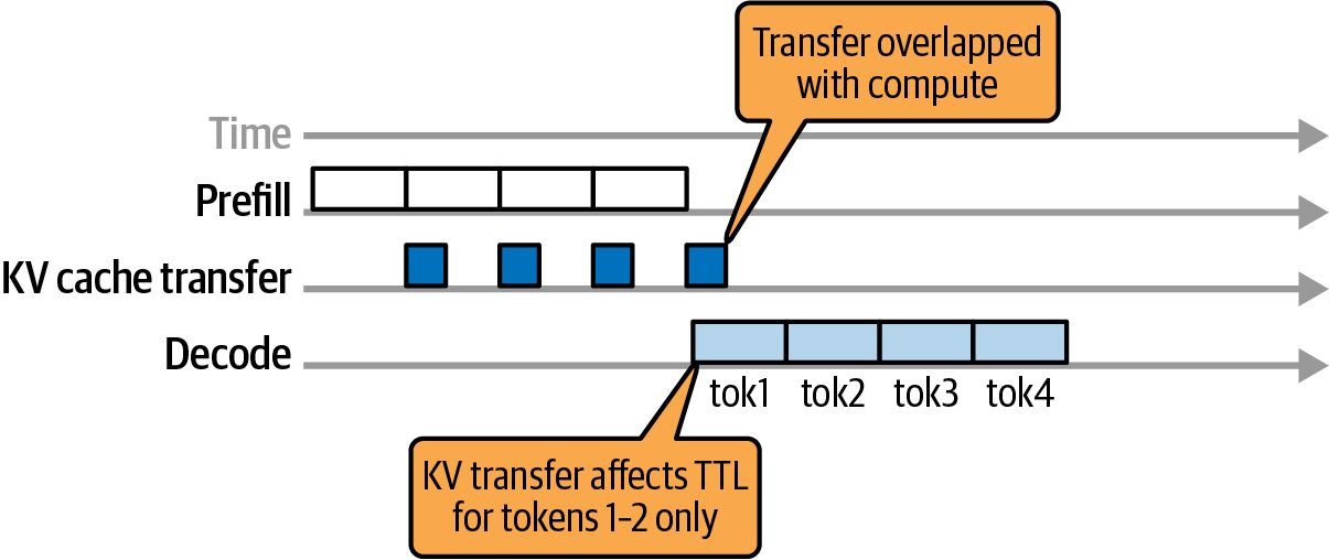
In the prefill stage, the model processes the entire input prompt—often thousands, tens of thousands, or even millions of tokens—in a single forward pass to produce initial hidden states as calculated by the LLM. It then populates the attention keyvalue (KV) cache for all tokens in the input prompt. Figure 15-1 shows how disaggre‐ gated prefill and decode share the KV cache and overlap KV transfers with computations.
Figure 15-1. Disaggregated prefill and decode sharing the KV cache and overlapping KV transfers with computations
In the decode stage, the model performs an autoregressive generation to predict each new token in the sequence. It does this by consuming the cached attention KV repre‐ sentations of all previously generated tokens.
664 | Chapter 15: Multinode Inference, Parallelism, Decoding, and Routing Optimizations
               Speculative decoding accelerates the decode process by pregenerat‐
               ing multiple tokens in a single batch. In parallel, it then verifies that
               the tokens are correct. This reduces the sequential nature of stan‐
               dard token-by-token autoregressive decoding. We’ll cover specula‐
               tive decoding in a bit.
Prefill-Decode Interference Traditionally, LLM inference systems colocate these two stages on the same nodes and simply batch all computations together. However, this naive approach leads to what’s commonly called prefill-decode interference. For instance, a long prompt prefill can occupy the GPU and delay time-sensitive decoding work for other requests—and vice versa. Colocating prefill and decode on the same nodes forces a single scheduling and resource allocation strategy for these two phases, which have very different character‐ istics. Prefill consists of large, parallel computations. In contrast, decode requires many small, sequential computations. As a result, systems have to either prioritize one phase’s performance over the other or over-provision hardware to meet both demands. With a disaggregated prefill and decode architecture, the prefill and decode phases are assigned to different GPU pools. This eliminates direct interference between the two workloads. The DistServe system, by disaggregating prefill and decode, reported up to 7.4× more goodput requests served within both TTFT and TPOT constraints (up to 12.6× tighter latency SLOs).
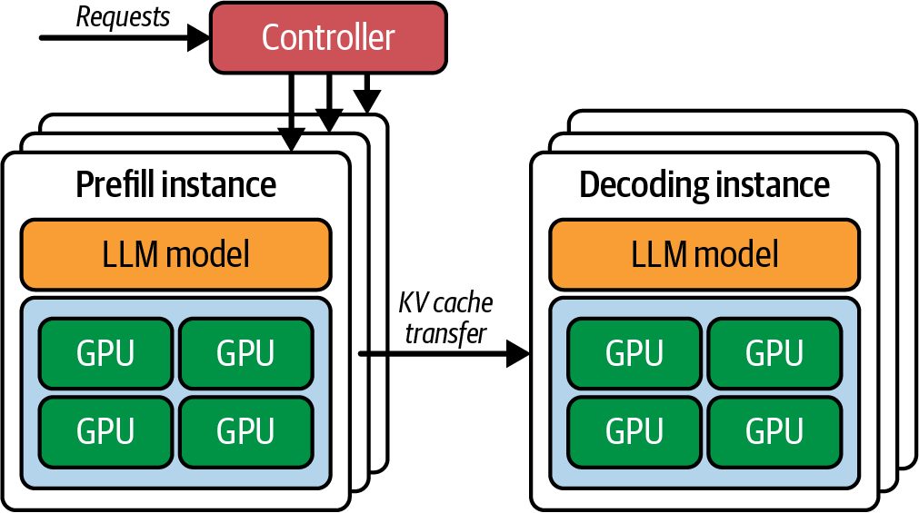
Scaling Prefill and Worker Nodes Independently If we can eliminate cross-phase interference, we can reduce resource “dead time” in which decode tasks are stalled behind long prefill computations—and vice versa. This way, GPUs spend more time doing more useful work and less time idling. This increases utilization and useful throughput at a given latency target (aka goodput). We can scale prefill and decode separately by dedicating one set of nodes to handle the prefill and another set of nodes to handle the decode. The two clusters communi‐ cate only when transferring the encoded prompt state, or attention KV cache, from the prefill workers to the decode workers, as shown in Figure 15-2. Here, you see separate GPU workers handling the prefill stage to process the input prompt—along with the decode stage to generate output tokens iteratively. The out‐ put of the prefill stage includes the KV cache for the prompt. It is transferred to the decode workers to generate the next tokens.
Disaggregated Prefill and Decode Architecture | 665
Figure 15-2. Disaggregated inference: Prefill pool (hidden state + KV) → KV handoff using NVLink/NVSwitch (intranode) or GPUDirect RDMA (internode) → Decode pool
By dedicating separate GPU pools, the system keeps both prefill and decode pipelines busy in parallel. In practice, disaggregation has been shown to significantly improve throughput under strict latency constraints. Some studies show that large gains are possible, but results range from moderate improvements to several times higher goodput once the prefill and decode stages are separated. The results greatly depend on the workload and network fabric. This separation allows each stage to be optimized and scaled independently for throughput or latency. Prefills can be batched aggressively on the prefill GPUs to maximize throughput without burdening the decode performance (e.g., increased decode latency). Also, with separate clusters we can tune parallelism settings, instance counts, and scheduling policies specific to each phase.
Impact on Latency (TTFT) and Throughput (TPOT) Decode GPUs can run at lower batch sizes—or with specialized scheduling—to mini‐ mize time per output token (TPOT) for streaming generation. For example, you can use a scheduler that prioritizes urgent decode tasks to avoid queuing delays. This separation works well because each phase has different performance expecta‐ tions. Time to first token (TTFT) for the prefill stage is optimized for low latency, while the decode stage prioritizes low time per output token (TPOT) and stable streaming latency. End-to-end throughput is largely determined by concurrency and scheduling. In traditional setups, one had to compromise between TTFT and TPOT per-token latency. Disaggregation allows both SLO targets to be met simultaneously.
666 | Chapter 15: Multinode Inference, Parallelism, Decoding, and Routing Optimizations
               Monitor NVLink and NIC utilization during KV transfer and all-
               to-all phases. The goal is to overlap cop and compute using sepa‐
               rate streams and events.
The KV handoff incurs minimal additional latency because the communication uses high-bandwidth interconnects for multi-GPU and multinode transfers. These inter‐ connects include NVLink, NVSwitch, InfiniBand, and Ethernet (RoCE on Ethernet) using GPUDirect RDMA. For instance, multinode clusters with ConnectX-8 SuperNICs (800 GbE-class) provides up to 800 Gb/s per port with GPUDirect RDMA. This greatly reduces KV transfer time compared to host-mediated communi‐ cation paths. Additionally, it’s recommended to deploy 1 NIC per GPU to optimize prefill-decode disaggregation and improve MoE all-to-all performance.
KV Cache Data Transfer and NIXL Disaggregated systems use a connector or scheduler to transfer the prompt’s inter‐ mediate results (the final hidden state and the KV cache) from the prefill workers to the decode workers once the prompt processing is done. This handoff incurs some communication overhead, but if the cluster’s interconnect is high-bandwidth (e.g., NVLink or InfiniBand), this overhead is small compared to the gains from eliminat‐ ing resource contention. In practice, NVIDIA’s NIXL library minimizes transfer overhead by selecting NVLink/NVSwitch, RDMA, or host-staged paths automatically based on topology and policy. For example, NVIDIA’s NIXL library, introduced in Chapter 4, will auto‐ matically select the fastest available path to transmit the KV cache. NIXL integrates with frameworks and inference engines, including Dynamo and vLLM. The NIXLvLLM integration is shown in Figure 15-3. Specifically, LMCache and NIXL are integrated in vLLM’s disaggregated prefilling as the supported path. NIXL is also used by NVIDIA Dynamo and TensorRT-LLM to transport KV cache data using peer-to-peer GPU interconnects and RDMA. Within a node, NIXL performs device-to-device transfers over NVLink and NVSwitch without host staging. Across nodes, NIXL uses GPUDirect RDMA over InfiniBand or RoCEv2 to avoid host copies. These paths keep KV cache handoff latency low even for multigigabyte payloads.
Disaggregated Prefill and Decode Architecture | 667
Figure 15-3. KV cache data transfers with NIXL in the vLLM inference engine; Intra‐ node: NVLink/NVSwitch (device-to-device); Internode: GPUDirect RDMA (InfiniBand/ RoCEv2) using ConnectX-class NICs
Placement of prefill and decode workers should follow the fabric. Same node place‐ ment keeps KV transfers on NVLink and NVSwitch via CUDA peer access, while cross-node placement should use GPUDirect RDMA over InfiniBand or RoCEv2. NVIDIA Dynamo integrates with NIXL to move KV cache between GPUs, CPU memory, and storage across nodes, and vLLM integrates through LMCache and NIXL for disaggregated prefilling.
                     When the fabric or virtualization layer prevents direct peer access,
                     NIXL can fall back to host-staged paths, which are nonoptimal.
                     Always validate end-to-end KV transfer time on your deployment.
Deploying Disaggregated Prefill and Decode with Kubernetes In an advanced deployment, a cluster orchestration system like Kubernetes can dynamically shift the GPU pool allocations—or scale the pools out separately—based on load and input characteristics. For instance, if many users arrive with superlong prompts and relatively small outputs (e.g., large-document summarization use cases), Kubernetes can temporarily shift the allocation to use more GPUs in the prefill pool. This will decrease the number of GPUs allocated to the decode phase. In contrast, if many users arrive requesting superlong outputs (e.g., long reasoning chains, “think step-by-step,” etc.), more GPUs can be shifted to the decode pool. In both cases, new instances can be scaled out for each worker type.
668 | Chapter 15: Multinode Inference, Parallelism, Decoding, and Routing Optimizations
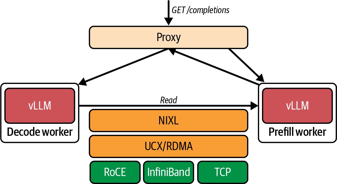
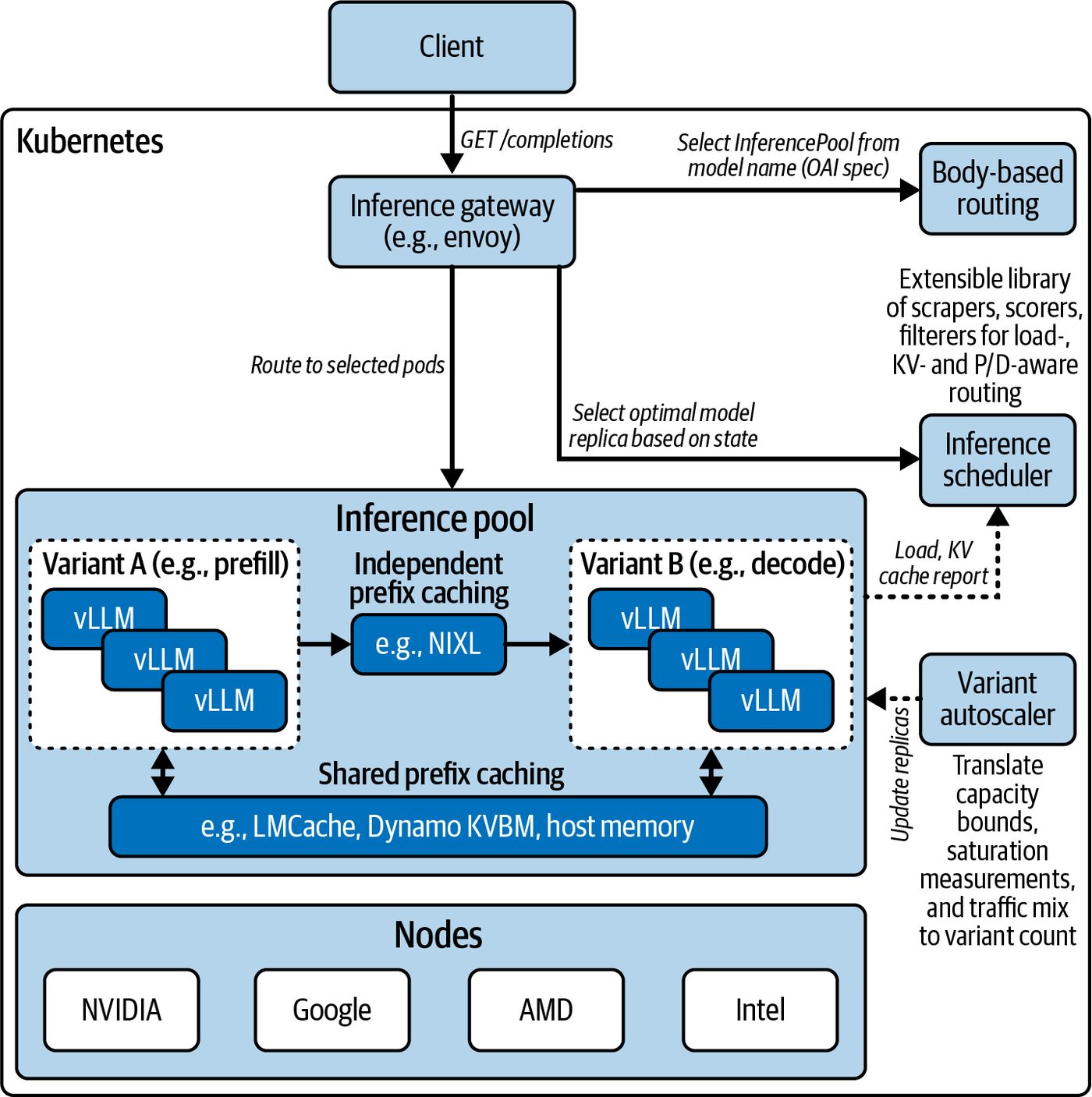
Figure 15-4 shows a distributed, Kubernetes-based vLLM cluster of separate prefill and decode workers using the open source llm-d project. vLLM implements disaggre‐ gated prefilling by running two instances and handing off KV using LMCache and NIXL, but llm-d extends this with Kubernetes native orchestration for disaggregated serving and KV-aware routing. This diagram shows a component called the variant autoscaler, which is responsible for updating the number of replicas for the prefill and decode workers in the pool.
Figure 15-4. Kubernetes-based vLLM cluster of separate prefill and decode workers using the open source llm-d project; variant autoscaler tunes prefill/decode replica counts based on the prompt-response mix; KV moved using LMCache and NIXL
Disaggregated Prefill and Decode Architecture | 669
                     In modern inference deployments, all nodes can perform both pre‐
                     fill and decode functionality since they all share the same runtime
                     and code base (e.g., vLLM, SGLang, NVIDIA Dynamo, etc.). It’s up
                     to the cluster orchestrator to assign them a specific role, either pre‐
                     fill or decode, statically upon startup—and dynamically throughout
                     the worker’s lifecycle.
Overall, a disaggregated prefill/decode architecture provides a foundation for highthroughput, low-latency LLM serving. It does introduce complexity, however, as intermediate data must be transferred and managed—on the order of a few gigabytes for the KV cache of a long prompt. And scheduling is more involved, but the benefits of utilizing hardware efficiently are significant at ultra scale.
                     Chapters 17 and 18 dive deeper into additional techniques for dis‐
                     aggregated PD, including advanced scheduling, routing, and
                     deployment optimizations.
Parallelism Strategies for Serving Massive MoE Models Serving massive MoE models efficiently requires multiple forms of parallelism due to limited GPU memory. We break down the key parallelism strategies, including ten‐ sor, pipeline, expert, data, and context parallel. We’ll also discuss how they can be combined to distribute an LLM across many GPUs. Table 15-1 provides a high-level summary of these strategies, their typical use, and a description of each strategy in more detail as they relate to inference.
Table 15-1. Parallelism strategies for LLM inference
Parallelism    Partition basis     Use case                 Pros                      Cons
strategy
Tensor         Within each layer   Single model is too      Near-linear speedup on    Frequent communication at each
parallelism    (split neural       large or you need to     compute-bound layers      layer (all-reduce)
               network weight      speed up heavy           Reduced overhead due to   Requires high-bandwidth
               matrices across     compute within           overlapping all-reduce    interconnect (NVLink/NVSwitch)
               GPUs)               layers across multiple   communication with        Less efficient across nodes and
                                   GPUs                     computation               slow networks due to high
                                                                                      latencies
                                                                                      (Recommended to keep tensor
                                                                                      parallel groups within a single
                                                                                      node)
670 | Chapter 15: Multinode Inference, Parallelism, Decoding, and Routing Optimizations
Parallelism   Partition basis      Use case                Pros                             Cons
strategy
Pipeline      Different layers     Extremely deep          Allows distribution of model     Adds pipeline fill/flush latency
parallelism   on different GPUs    models that don’t fit   state                            (bubbles)—not helpful for one-
              (the model is        on one GPU              Uses microbatching to            token-at-a-time decoding
              sliced by layer      Memory scaling          process multiple tokens from     More complex to implement and
              sequence)            across layers           different users/requests         higher activation memory
                                                           concurrently                     footprint (must store intermediate
                                                           Multiple layers can be           activations between pipeline
                                                           processed in parallel for long   stages)
                                                           sequences (improves
                                                           throughput for large batches
                                                           or long inputs)
Expert        Different MoE on     Massive MoE models      Enables virtually unlimited      High runtime communication
parallelism   different GPUs       with many experts       model size—total                 overhead (all-to-all) at each MoE
              (sparse activation   Needed to shard         parameters scale with            layer
              per token)           model parameters        number of GPUs                   Potential load imbalance if gating
                                   across GPUs             Each GPU computes only a         is uneven
                                                           fraction of tokens (sparse       Each GPU must have enough work
                                                           compute)                         (tokens) per expert to amortize
                                                           High parameter count boosts      communication
                                                           model capacity/quality
Data          Replicate the        Scaling out             Nearly linear throughput         No latency improvement for
parallelism   entire model on      throughput (more        scaling                          individual queries (aka per-query
              multiple GPUs,       concurrent requests)    Simple to implement (no          latency)
              serving different    once model              model partitioning needed)       Multiplies memory usage (each
              requests on each     deployment is fixed                                      replica uses full memory)
                                   Multi-instance                                           Must handle consistency if
                                   serving for many                                         stateful (e.g., caches) or use
                                   users                                                    stateless model calls
Context       Partition the        Ultralong sequences     Achieves near-linear             Requires custom attention
parallelism   input sequence       (e.g., 100k+ tokens)    speedup for long context         algorithms to handle attention
              tokens across        to reduce prompt        prefill                          across partitions
              GPUs at each         latency and memory      Enables processing contexts      Adds communication per layer for
              layer                per GPU                 that exceed one GPU’s            boundary tokens
                                                           memory by splitting KV           Beneficial for very long contexts
                                                           cache                            (100k+ tokens) due to additional
                                                                                            communication overhead
                    For intranode TP on Blackwell NVL72, prefer keeping TP groups
                    within a single NVSwitch domain; extend inter-rack only when
                    topology permits to avoid extra hops.
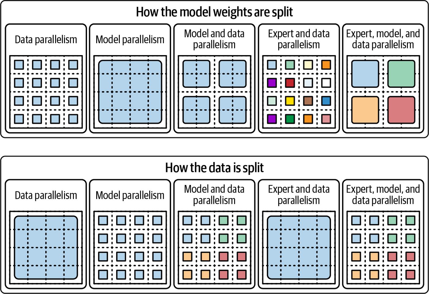
These parallelism strategies define how the model weights and data are split over the GPUs. Figure 15-5 shows how they are split up for the different parallelism strategies— as well as common combinations of strategies.
Parallelism Strategies for Serving Massive MoE Models | 671
Figure 15-5. Model weights and input data split over the GPUs
Tensor Parallelism Tensor parallelism (TP) splits the computations within each layer of the neural net‐ work across multiple GPUs. For instance, a large matrix multiply in a transformer layer can be partitioned by columns or rows—and computed in parallel on two or more GPUs. These GPUs then exchange their results by performing an all-reduce to aggregate their partial outputs. TP is commonly used when a model’s layers, called hidden layers, are too large to fit into a single GPU’s memory—or when we want to accelerate a single instance of a model by utilizing multiple GPUs for the same layer in parallel. It keeps all GPUs in lockstep for each layer’s computation, which requires extremely high inter-GPU bandwidth to be efficient. Ideally, TP runs on GPUs that are connected with high-bandwidth NVLink and NVSwitch interconnects. On multi-GPU Blackwell systems that use fifth-generation NVLink (up to 1.8 TB/s aggregate bidirectional GPU-to-GPU bandwidth and advanced network topologies), TP can scale efficiently across a node of 8–16 GPUs— or even up to 72 GPUs in the case of an NVL72 rack. Remember, within the GB200/ GB300 NVL72 racks, NVLink Switch provides about 130 TB/s of aggregate GPU bandwidth within the 72 GPU domain. This is a large amount of intra-rack bandwidth.
672 | Chapter 15: Multinode Inference, Parallelism, Decoding, and Routing Optimizations
TP provides near-linear speedups for compute-bound portions of the model as long as collective communications, such as the all-reduce of activations, are fast relative to computation. In inference, tensor parallelism is mainly applied to the large matrix multiplications of the attention projections and feed-forward multilayer perceptron (MLP) networks. Since the activations for one token are relatively small, those all-reduce communica‐ tions are not too costly on NVLink. As such, TP is a common strategy for splitting giant dense models across GPUs without approximating model weights. We mainly use TP to serve models in which single MoE experts or transformer layers are too large for a single GPU. However, we also use it when we want to reduce latency by parallelizing each layer’s computations across multiple GPUs. One must be mindful that beyond a certain scale, however, TP efficiency drops— especially when using it across nodes or racks running over InfiniBand or Ethernet. In practice, it’s best to use TP for intranode communication—or between nodes in an NVLink domain. Modern multi-GPU racks like NVIDIA’s GB200/GB300 NVL72 allow TP to be used at a much larger scale without saturating interconnect bandwidth. NVLink Switch extends the NVLink domain across the rack to 72 GPUs per NVL72. NVLink Switch Systems can scale an all-to-all, fully connected NVLink fabric across up to 8 racks, or 576 GPUs (576 GPUs = 8 racks * 72 GPUs per rack). This enables large-scale parallel‐ ism strategies, not just inside a single NVL72 but also across multiple racks. For instance, in an 8-rack topology, you can increase to 576-way tensor parallelism using the 576 GPUs across 8 racks (576 GPUs = 8 racks × 72 GPUs per rack.)
                While it’s possible to extend TP across racks, it’s recommended to
                choose your TP group sizes with topology-awareness in mind and
                within a single NVLink/NVSwitch island whenever possible. This
                will avoid unnecessary inter-rack switch latency and help to
                increase overall system efficiency.
Pipeline Parallelism Pipeline parallelism (PP) partitions the model layer-wise across different GPUs. For example, in a 60-layer transformer-based model, GPU 0 might hold layers 1–20, GPU 1 holds layers 21–40, and GPU 2 holds layers 41–60. When processing a sequence of tokens, the data flows through the GPUs in sequence such that GPU 0 computes layers 1–20, then passes its intermediate activations to GPU 1 for layers 21–40, and so on. This allows models that are too deep to fit on one accelerator to be distributed.
Parallelism Strategies for Serving Massive MoE Models | 673
In inference, PP can improve throughput by partitioning the model across multiple batches—similar to an assembly line. During the prefill phase, which processes a long sequence of input tokens, PP achieves high GPU utilization by streaming different portions of the sequence into the layers in staggered fashion. In contrast, during the decode phase, generating one token at a time, pure PP offers less benefit since each new token must still pass through the pipeline stages sequen‐ tially. This creates pipeline bubbles, or idle periods, in which earlier stages wait for later ones to finish for each and every token. To reduce pipeline bubbles, implementations use microbatching, which allows the pipeline to process multiple tokens from different requests concurrently. Still, pipe‐ line parallelism primarily helps with memory scaling by enabling very large models to split layers among GPUs. It also helps throughput—especially when handling large batch sizes or long inputs. PP tends to increase end-to-end latency for a single item due to transfer overhead between pipeline stages. As such, PP is usually chosen for model capacity reasons— rather than latency reasons. This is because it can fit the model into memory. The slight latency hit is acceptable when no single GPU can hold the whole model. Additionally, PP is often used in combination with other parallelism strategies like TP to balance memory and speed. When serving large MoE models, one might use pipe‐ line parallelism across 2–4 GPUs to split the deep layer stack—while relying on TP to handle the wide, intralayer compute.
                     PP splits the model across layers, and TP splits the model within
                     layers. TP is mainly used for models with layers or experts that are
                     too wide for a single GPU, while PP is primarily used for models
                     that are too deep to fit into a single GPU. Note that TP and PP can
                     be combined, which we’ll see in a bit.
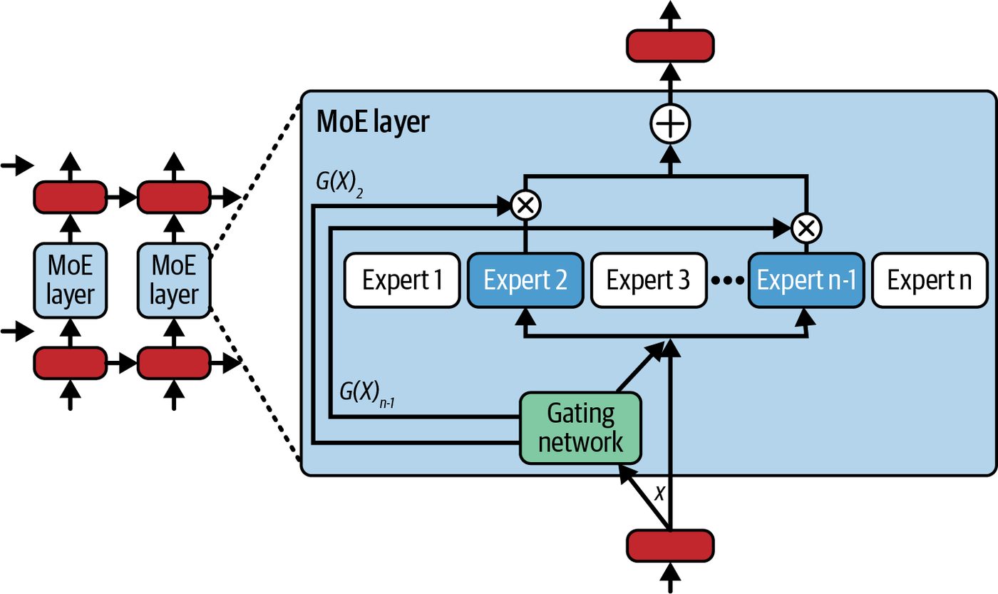
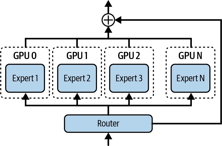
Expert Parallelism Expert parallelism (EP) is specific to MoE architectures. In an MoE layer, there are many expert networks, or feed-forward sublayers. For each input token, only one or a few experts are activated. This naturally lends itself to distributing different experts on different GPUs. For instance, if an MoE layer has 16 experts and we have 4 GPUs, each GPU could host 4 experts. During inference, when a token arrives at that MoE layer, its internal gating network will choose the top two experts, for instance, for that token. The token’s data is then sent to whichever GPUs own those two experts for processing. Then the results are combined back to generate the next token, as shown in Figure 15-6.
674 | Chapter 15: Multinode Inference, Parallelism, Decoding, and Routing Optimizations
Figure 15-6. Mixture-of-experts (MoE) communication (source: https://oreil.ly/pzn5t)
Implementing this requires an all-to-all communication pattern such that tokens (technically, their activation vectors) are dynamically shuffled between GPUs so that each token lands on the GPU of its assigned expert. After each expert computes its output for its assigned tokens, another all-to-all is performed to return the token out‐ puts back to their original order. This dynamic routing introduces a communication-heavy step at each MoE layer. This can become a performance bottleneck if not carefully optimized—especially as the number of experts/GPUs increases. The upside is that expert parallelism allows the total model capacity to scale almost linearly with the number of GPUs. Consider an MoE with 100 experts distributed across 100 GPUs. If each token acti‐ vates only two experts, the compute per token is similar to a smaller dense model. As such, expert parallelism is what allows some massive MoE models to be served at all since the model weights are sharded across many GPUs—and each GPU handles only a fraction of the tokens at any given layer.
               At scale, and with a properly balanced set of experts in an MoE
               model, all of the experts will likely be active simultaneously.
               So, while an individual token activates only a small number of
               experts, in aggregate across all tokens across all end users, all
               experts will be active, consuming and contending for all GPU
               resources concurrently.
Parallelism Strategies for Serving Massive MoE Models | 675
Efficient expert parallel inference requires careful load balancing—as well as highbandwidth interconnects, such as NVLink/NVSwitch for intra-rack communication and InfiniBand/RDMA for internode communication. Modern MoE inference frame‐ works use fast collective communication libraries like NCCL. It often helps to group multiple experts per GPU to reduce communication steps. Modern MoE inference often uses top-2 gating, in which each token is assigned to two experts. To reduce communication, you can group commonly paired experts onto the same GPU or compute node. For instance, if tokens use two experts, placing those two frequently paired experts on the same GPU or node means that many token assignments will stay on a single GPU or node, which will localize communica‐ tion traffic and reduce overhead. Another technique is to use top-1 gating, in which each token goes to only one expert. This will reduce the communication volume relative to top-2 gating described previously, which doubles the number of expert outputs. While top-1 gating is faster, it can lead to a lower model quality and uneven load.
                     Google’s GLaM introduced load-balancing losses (and gating noise)
                     to achieve balanced expert usage during MoE model training.
                     Building on this, researchers are exploring truly adaptive,
                     inference-time gating that uses real-time load metrics to reroute
                     tokens when an expert is overloaded. These improve utilization
                     without degrading quality.
                     However, in most production serving environments, top-2 gating
                     with a modest capacity factor—and occasional load-based expert
                     swapping or replication—remains the most common compromise
                     technique to balance both quality and performance.
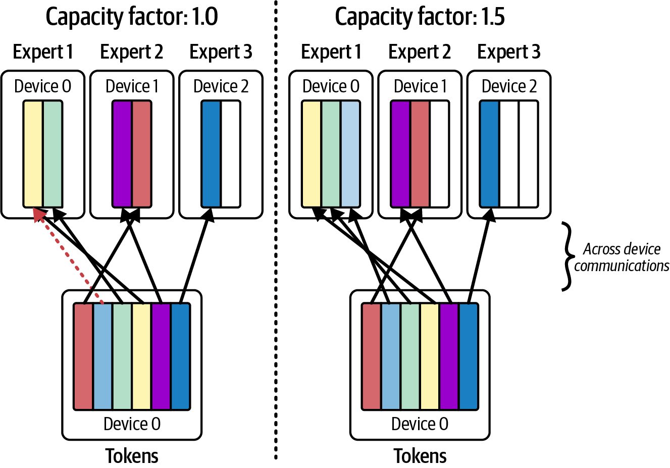
Many MoE LLMs use at least top-2 gating for better quality, good speed, and balanced load. Additionally, it’s important to place experts strategically—or even use backup expert replicas to avoid overloading experts. When experts become overloaded, or hot, they can become throughput bottlenecks if the gating network is disproportionately routing tokens to them. The straggler effect, as it’s called, requires that all expert computations be complete before they can pro‐ gress. As such, an overloaded expert that receives more work (tokens) than other experts will stall the inference pipeline. This will leave some experts, and their GPUs, idle while the other experts catch up. To prevent this, high-performance MoE serving systems expose a capacity factor parameter, typically set at 1.2–1.5× the average token load, which caps how many tokens each expert can process per batch. Tokens beyond that are routed to a secondchoice overflow expert—or queued for a second pass. This complements any
676 | Chapter 15: Multinode Inference, Parallelism, Decoding, and Routing Optimizations
load-balancing loss or gating noise used during training to encourage the MoE to assign tokens to experts uniformly. Some full-featured inference servers can also replicate hot experts onto multiple GPUs to split the load if necessary. This comes at a cost of additional GPU memory. We will see an example of load imbalance a bit later. The combination of inference-time spillover (capacity factor), training-time penalties (load-balancing loss and gating noise), and hot-expert replicas should smooth out the token-expert load distribution when capacity is reached—maximizing overall MoE inference throughput.
Data Parallelism In inference, data parallelism (DP) refers to replicating the entire model on multiple GPUs and assigning different incoming requests—or shards of a request batch—to each GPU. Unlike data parallelism in training, which keeps models in sync with gra‐ dient averaging, data parallelism in inference runs independent forward passes on each replica. This is the simplest way to scale out throughput. For instance, with DP, if one GPU can handle 10 requests per second, using 8 GPUs with 8 replicas ideally gives 80 requests per second of throughput—assuming the requests are independent. In practice, using data parallelism for inference requires spinning up multiple model-serving engines and load-balancing requests among them. When using DP, each GPU, or group of GPUs, handles a subset of queries from start to finish. The advantage is linear scaling of throughput and no inter-GPU communi‐ cation during inference since each replica runs in isolation. The disadvantages are significant, however. DP multiplies the memory requirement since each replica needs a full copy of model weights and cache. As such, serving a model with eight replicas uses 8× the GPU memory—and roughly 8× the hardware cost—compared to hosting the model on a single GPU. In practice, data parallelism is often combined with request batching and multistream execution on each GPU to maximize utilization. Each replica should ideally be stateless—or use synchronized caches to avoid consistency issues. It’s important to note that DP does not reduce latency for any single request. It does, however, improve throughput since there are more replicas available to handle requests—assuming the memory and compute resources are available and relatively free of contention.
Parallelism Strategies for Serving Massive MoE Models | 677
                    Because GPU memory is relatively scarce and expensive, DP is
                    usually worthwhile for inference only when your throughput needs
                    are very high—or if you can combine DP with other parallelism
                    approaches, such as TP and PP.
For inference, DP is often used in combination with other parallelism approaches, such as TP and PP, due to the additional memory and cost requirements of DP. For example, if a model must be spread across eight GPUs due to memory limitations, it should use DP with TP, PP, or EP—or even all of them together—to create fourdimensional (4D) parallelism (add in context parallelism (CP), and you’re using 5D parallelism!). Specifically, you can use DP with TP to deploy two large, 8-GPU model replicas using two DP groups of eight GPUs. This will double the throughput and shard each of the large model replicas across eight GPUs within its layers using TP. In a massive inference cluster, you can dedicate a large number of GPUs and nodes to serve multiple copies of the large model to handle high request volumes. DP is partic‐ ularly useful when throughput needs to scale beyond what a single model instance can provide. In practice, production systems often run many DP replicas of the large model to meet traffic demands.
                    Modern inference servers treat each replica as a separate model
                    instance behind a load balancer. This requires careful request rout‐
                    ing, but it’s relatively straightforward compared to other complex
                    model-sharding methods.
Context (Sequence) Parallelism Context parallelism (CP) is more of a specialized strategy that partitions a single sequence of tokens across multiple GPUs. This technique benefits extremely long context inputs on the order of tens of thousands and millions of tokens. These would otherwise be too slow or memory-heavy or simply not fit on a single GPU. The idea behind CP is to split the sequence into chunks and have different GPUs han‐ dle different parts of the sequence in parallel at each layer. The GPUs exchange only the necessary information at the boundary between chunks of the sequence. CP handles contexts larger than a single GPU’s memory by splitting the KV cache across GPUs. It also reduces prompt-processing latency roughly in proportion to the number of GPUs used. As such, CP can achieve near-linear speedup for very long context prefill runs by using multiple GPUs to perform the prefill for a long context in parallel.
678 | Chapter 15: Multinode Inference, Parallelism, Decoding, and Routing Optimizations
The challenge with CP is that transformers have global self-attention such that every token attends to every earlier token. Naively splitting the sequence would require lots of information exchange between GPUs to compute attention across the partition boundary. CP methods use clever schemes like ring parallelism and blocked attention to reduce the quadratic self-attention communication time complexity—and limit each GPU to attending mostly within its partition of the context as well as a small amount of chunk-boundary data. In effect, each GPU handles a subset of positions in the input sequence for each layer. They pass intermediate results around in a pipelined fashion—often arranged in a ring. CP is analogous to pipeline parallelism but along the sequence-length dimen‐ sion instead of the layer dimension. Context parallelism excels at prefill for very long inputs by slicing a document into segments, allocating segments across multiple GPUs, and processing each segment concurrently. This reduces prompt‐processing time roughly in half for every dou‐ bling of GPUs—with only a bit of overhead for cross‐segment attention at the boundaries. In short, while CP doesn’t speed up the sequential, token‐by‐token decode phase, it can shorten TTFT for extremely long prompts. It does this by distributing the atten‐ tion KV cache across devices such that each GPU stores only its segment’s cache. CP also lets you handle contexts larger than what a single GPU can fit into memory.
               Context parallelism requires an attention implementation that
               communicates across partitions. This adds extra per-layer commu‐
               nication. As such, for short prompts, CP often adds outsized over‐
               head. But for very long inputs and strict TTFT goals, CP can
               reduce prefill latency and memory per GPU. Measure both prefill
               speed and accuracy for your maximum context.
Hybrid Parallelism In practice, serving massive MoE LLMs uses a combination of the previous parallel‐ ism strategies. Today’s LLM models are so large and complex that no single paralleli‐ zation method is sufficient. Figure 15-7 shows a hybrid parallel configuration using four GPUs.
Parallelism Strategies for Serving Massive MoE Models | 679
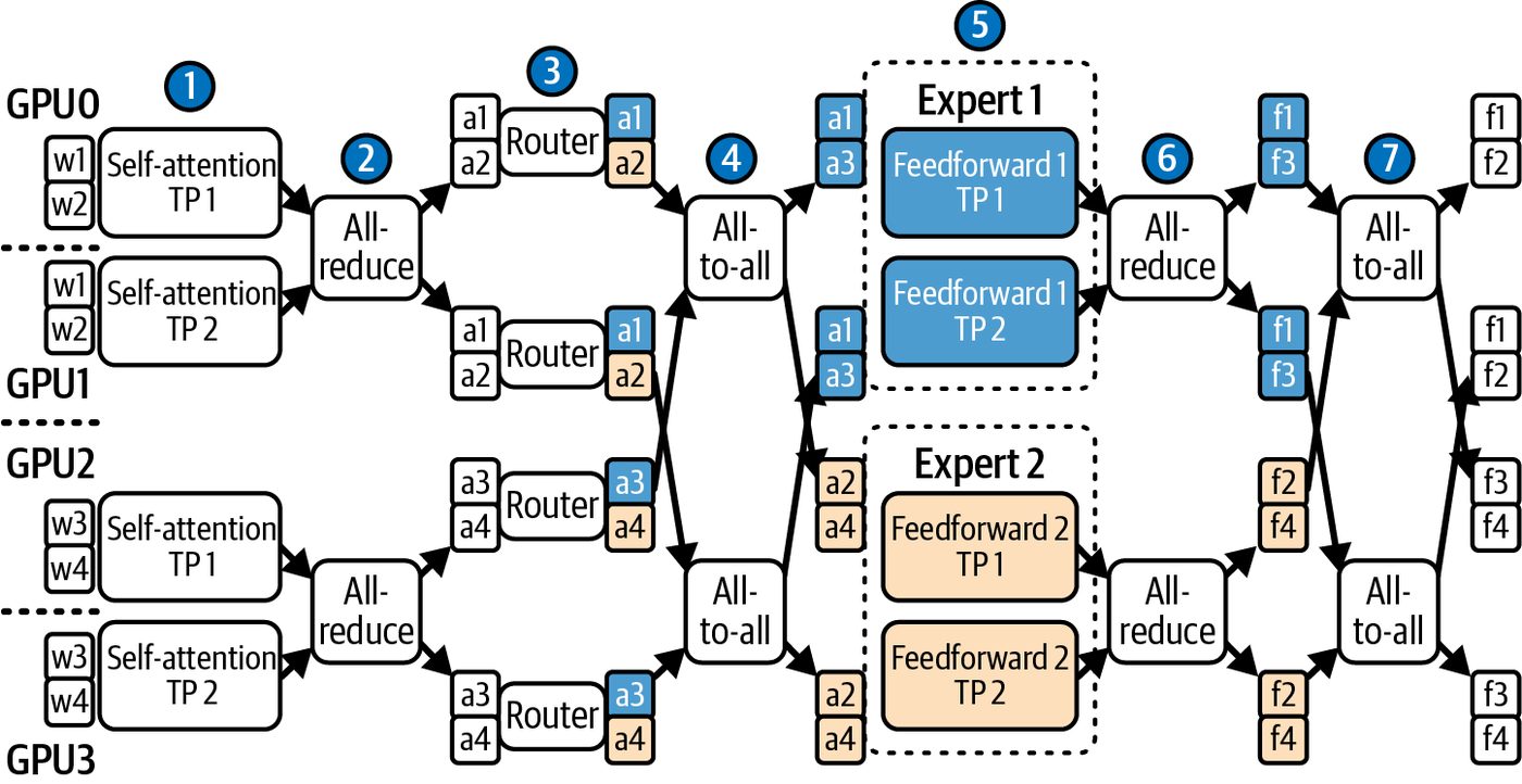
Figure 15-7. High-level diagram of a 4 × 2 × EP hybrid parallel combination (source: https://oreil.ly/q1AEf)
Here, we are using four pipeline stages (one per GPU) and two-way tensor parallel‐ ism. The tokens are routed across two experts using expert parallelism. This is called a 4 × 2 EP hybrid parallel strategy. Let’s go even larger and create logic groups of GPUs. For example, consider a cluster of 64 GPUs. We can group the GPUs into 16 groups of 4 GPUs each. Using an MoE with 60 layers and 64 experts, we can use 4-way pipeline parallelism with 15 layers per stage. This splits the depth of the model. Then, within each stage (15 layers), we can use 2-way TP to split the heavy matrix multiplies within each layer. This splits the width of the model. For the MoE layers, you can use EP to spread 16 experts per group using top-2 gating. This will send tokens to, at most, two GPUs in the group. Finally, data parallelism can deploy two such 64-GPU replicas to double your system’s throughput. This is just one configuration. In practice, you’ll need to experiment with different combinations of parallelism strategies. Your profiling tools will help you find the right balance. Specifically, you can use Nsight Systems for end-to-end traces and Nsight Compute for kernel-specific GPU metrics.
                     Remember to always verify interconnect traffic, Tensor Core uti‐
                     lization, and other performance-enhancing mechanisms before and
                     after making each change.
680 | Chapter 15: Multinode Inference, Parallelism, Decoding, and Routing Optimizations
The guiding principle is to use TP up to the point of diminishing returns—usually within a node or in a tightly coupled unit like an NVL72 chassis. You would then use pipeline parallelism minimally—just enough to fit the model in memory. Then, you want to maximize EP to distribute MoE parameters across experts and GPUs. Finally, you add data parallel replicas to improve throughput as you scale to more and more end users and concurrent inference requests (CP can be optionally layered on top if extremely long inputs are expected). We also want to align parallelization with our hardware topology. For instance, if using an NVL72 system, all 72 GPUs are fully connected using NVLink and NVSwitch. In this case, you can form TP and EP groups within the 72 GPU NVLink domain. However, TP groups that approach the full domain will often see diminish‐ ing returns from the all-reduce latency. As such, many production systems keep TP groups smaller and topology aware—even inside NVL72. In contrast, a smaller cluster of two 8-GPU nodes connected with InfiniBand has full NVLink connectivity only within each node—with cross-node traffic traveling along the InfiniBand fabric. In such environments, it’s best to keep TP local to each 8-GPU node—and avoid internode parallelism if possible to avoid the higher latency and lower bandwidth of internode communications. In the next sections, we discuss higher-level optimizations that can be combined with these parallelism strategies to achieve even faster inference on multinode clusters. As we shall see, a well-designed serving system will combine many of these high-level and low-level techniques.
Speculative Decoding and Parallel Token Generation Techniques One of the fundamental performance challenges in LLM inference is the sequential nature of decoding. Remember that after the initial prompt is processed during pre‐ fill, the model typically generates one token at a time. Each token’s computation depends on the result of the previous token, so this is difficult to parallelize as it’s inherently a serial process, which introduces a latency bottleneck—even with the lat‐ est, fastest GPUs. Generating hundreds of tokens sequentially can take on the order of seconds for massive models on modern GPU hardware. In this section, we discuss several techniques to accelerate the decode stage. Some of these techniques involve generating multiple tokens per inference step, while others reduce the number of sequential inference steps altogether. Speculative decoding traditionally pairs a small, fast “draft” model that proposes sev‐ eral tokens in one batch with a larger “target” model that then validates each candi‐ date. This trades a second inference pass for parallel generation to achieve higher,
Speculative Decoding and Parallel Token Generation Techniques | 681
multitoken throughput. However, running two separate models adds deployment complexity and can still stall inference when the verification pass becomes a bottleneck. Medusa simplifies this by attaching multiple lightweight decoding heads directly to a single LLM. At each step, these heads use a tree-based attention mechanism to con‐ currently generate and verify several token candidates within a single forward pass. This unified design of Medusa avoids cross-model token transfers and achieves large speedups without sacrificing the quality of the token generation. By consolidating draft-and-verify into a single-model pass, Medusa is an improvement over conven‐ tional two-model speculative decoding techniques. Let’s take a closer look at some of these techniques.
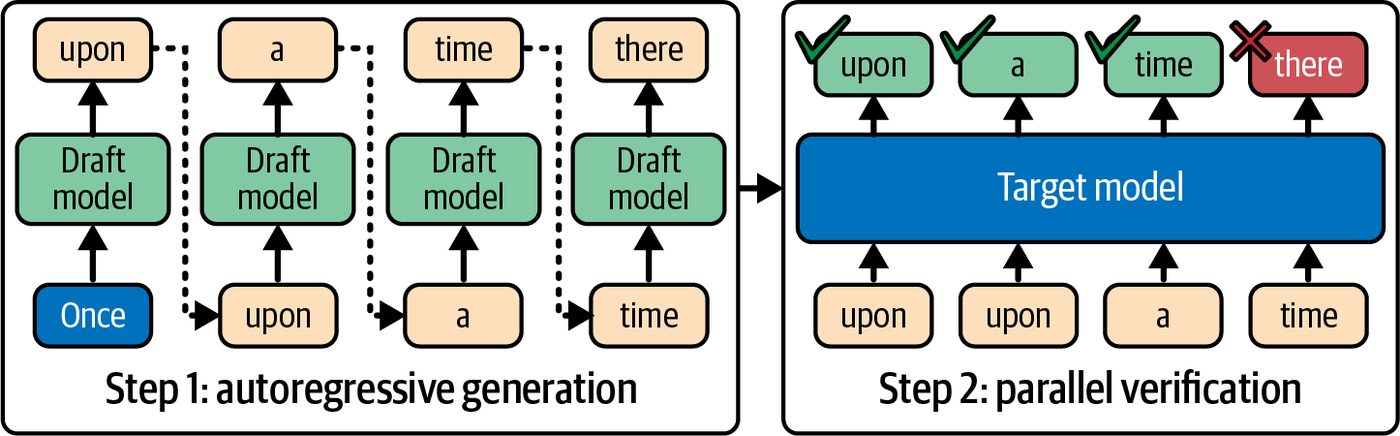
Two-Model, Draft-Based Speculative Decoding and EAGLE Speculative decoding is a technique that trades extra work on a small model to save time on the expensive large model. The idea is to run a lightweight “draft” LLM alongside the main LLM. The draft model is faster and generates a batch of k tokens speculatively beyond the current context. The big model, called the target model, then validates the draft tokens by predicting next-token probabilities for the entire k-token sequence in a single batch sent to the GPU. By handling all k tokens at once, the target model increases arithmetic intensity by performing more computations per byte of data transferred. This results in effi‐ cient and fast verification of the draft sequence tokens. If the target model’s output agrees with the draft model’s k proposed tokens, then we have effectively generated k tokens in the same time that a large model would have generated a single token. If the large model’s verification diverges from the draft model’s prediction at any token in the sequence of k tokens generated by the draft model, the speculative tokens beyond that point are discarded. At least one gen‐ erated token will be kept in each step because the verification procedure always accepts the first token from either the draft or the target model. Once the target model’s corrected token is used and decoding continues, a new specu‐ lative decoding cycle can start from that point. Figure 15-8 shows a small draft model predicting multiple tokens ahead. Then the target (big) model verifies these tokens one by one. Over time, speculative decoding reduces the overall number of one-by-one, sequen‐ tial invocations needed by the large model. In theory, it provides a theoretical k× speedup, where k is the number of tokens generated by the draft model. In practice, with overhead and occasional speculative-token rejections, the gain is more like a 2× speedup.
682 | Chapter 15: Multinode Inference, Parallelism, Decoding, and Routing Optimizations
Figure 15-8. Speculative decoding with a draft (small) for decoding and a target (large) model for multitoken verification
The draft model must be chosen to have reasonably high fidelity to the large model’s distribution. This means that the draft model’s predictions should have high overlap with the large model’s likely outputs. If the draft frequently guesses wrong, specula‐ tive decoding provides little benefit and wastes compute. If it often predicts tokens that the larger target model would not, many speculative tokens will be rejected. This will waste compute time. The draft model must also be much faster than the large model—typically by a factor of 4× or more—for speculative decoding to provide a practical performance improve‐ ment. A common strategy is to use a distilled version of the main model—or a smaller model fine-tuned on the same data so that its outputs correlate well.
                The draft model must use the same tokenizer and vocabulary as the
                large model. This is sometimes overlooked, and it will lead to poor
                results.
The draft model generates tokens using the same prompt and perhaps a higher tem‐ perature to increase the chance of matching one of the large model’s probable contin‐ uations. Meanwhile, the target model skips ahead and processes all of the draft tokens in one single batch. Under the standard speculative decoding acceptance procedure, the target model’s output distribution is preserved. As such, the final samples match the large model’s distribution when sampling settings are aligned. If the draft diverges, the target mod‐ el’s verification rejects those tokens and correctness is maintained. The only differ‐ ence is that up to k number of target-model calls are avoided when the small model guesses correctly for these speculative tokens. Speculative decoding can be implemented in a variety of ways. Most modern LLM inference engines like vLLM, SGLang, and TensorRT-LLM have built-in support to
Speculative Decoding and Parallel Token Generation Techniques | 683
coordinate draft and target model generation. Empirically, speedups around 1.5–2.5× are common, and higher gains are possible with careful batching and draft model design.
                     In PyTorch, the operation torch.nn.functional. scaled_ dot_
                     product_attention auto-selects the optimal backend (FlashAtten‐
                     tion or a cuDNN kernel) based on device generation, shapes, mask,
                     and dtype. You can pin a backend using torch.nn.attend
                     ion.sdpa_kernel() with an explicit SDPABackend type. It’s impor‐
                     tant to verify that the fused backend is active when benchmarking
                     LLM decoding, for instance.
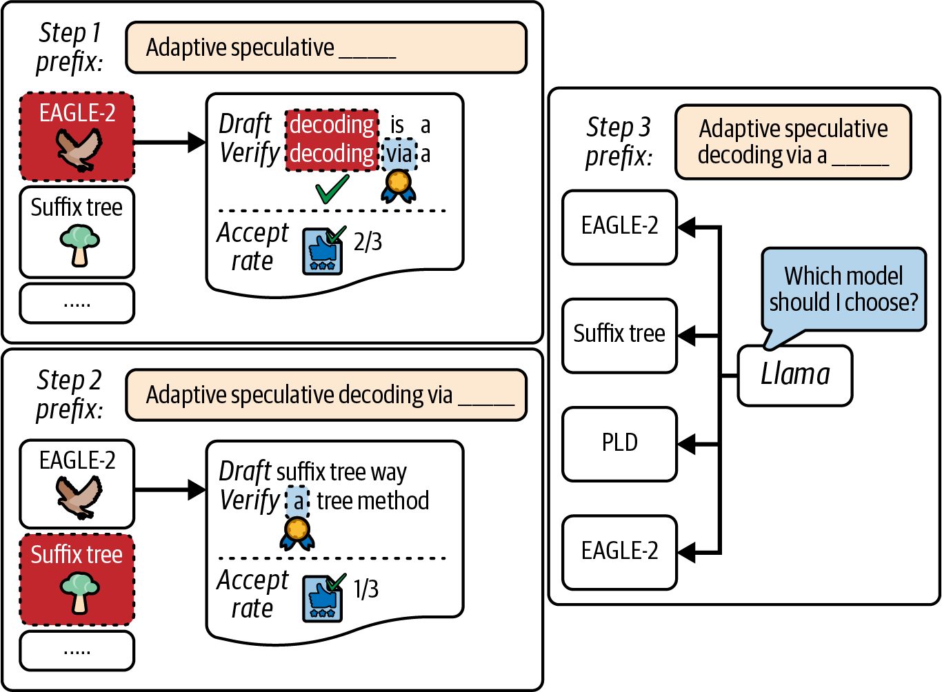
For instance, the Extrapolation Algorithm for Greater LLM Efficiency (EAGLE) algo‐ rithm rethinks speculative decoding by operating at the feature level rather than the token level. EAGLE uses a one-step extrapolation of the large model’s own intermedi‐ ate representation to predict the next token’s features. This resolves uncertainty and achieves higher acceptance rates. EAGLE reported up to about 3.5× speedup over vanilla decoding for a 4-token draft while preserving the large model’s output distribution. EAGLE approaches the theo‐ retical limit of its draft depth in favorable environments. And it shows that, with innovative techniques, speculative decoding can reduce decoding time even further— and preserve output quality at the same time. EAGLE-2 extends EAGLE by introducing a context-aware dynamic draft tree of pos‐ sibilities. While EAGLE achieved up to 3.5× speedup versus vanilla decoding in some evaluations, EAGLE-2’s approach reported speedups of about 20%–40% faster than EAGLE depending on the task and model. With EAGLE-2, the draft model generates a branching set of token sequences, which further increases parallelism in the verifi‐ cation step. This is shown in Figure 15-9. EAGLE-3 continues to improve on earlier versions, EAGLE-1 and EAGLE-2, by pre‐ ferring direct token prediction and fusing multi-layer features. EAGLE-3 reports up to 1.4× improvements over EAGLE-2 in certain tasks—and up to 6.5× speedups over non-optimized baseline variants. In EAGLE-1 and EAGLE-2, the draft model pre‐ dicts internal feature vectors which are then decoded to tokens. These earlier EAGLE methods worked by guessing internal features, essentially—and then mapping them to tokens. EAGLE-3 skips the feature-level prediction step and predicts the draft tokens more directly. However, it still uses internal features but fused into multiple layer representa‐ tions (lower, middle, upper) to guide the draft predictions. This is in contrast to using just the top layer. This makes EAGLE-3 more streamlined and less constrained—allow‐ ing better scaling.
684 | Chapter 15: Multinode Inference, Parallelism, Decoding, and Routing Optimizations
Figure 15-9. Speculative decoding with EAGLE-2 (source: https://oreil.ly/uG07b)
Another technique is dynamic depth decoding, which can adaptively skip layers that minimize the impact on output quality. Other techniques that reduce computations include skipping every Nth transformer layer, using lower precision (e.g., FFP8 and NVFP4) for the draft model, and using a smaller hidden size temporarily for the draft stage.
               Some research prototypes offer modes that skip portions of the
               network or reduce precision during decoding to trade accuracy for
               speed. As of this writing, these are not universally available in pro‐
               duction models, so always validate quality and speed on your target
               tasks before enabling any such mode.
Future LLMs might include an optimized “fast-generation” mode. For example, a model might have alternate lightweight layers or a configuration for reducedprecision decoding. This built-in optimization would allow the model to skip computations.
Speculative Decoding and Parallel Token Generation Techniques | 685
Single-Model Self-Speculative Decoding Another approach to speculative decoding is to avoid using an external draft model altogether and use the larger target model to both draft and verify its own outputs by selectively skipping some computations. One such method is self-speculative decod‐ ing, also called the draft-and-verify scheme. With self-speculative decoding, the large target model generates k tokens using a fast, approximate pass. For instance, it can choose to run only half of its layers—and possi‐ bly in reduced precision—for each new token. It would skip every other layer. This produces draft output much like the smaller draft model would. And it can approach similar speedups when acceptance rates and draft depth are favorable. This produces draft output much like the smaller draft model would—and achieves a similar 2× speedup as well. Then, in a second stage of self-speculative decoding, the target model performs a full forward pass to verify those k tokens in one go. If they all match, then we save execut‐ ing half the layers for those tokens. If not, we simply fall back to the traditional specu‐ lative approach by accepting tokens up to the mismatch and proceeding normally. Because it’s the same model doing both draft and verification in self-speculative decoding, no separate model needs to be trained, maintained, or loaded into memory at runtime. The challenge is finding a good way to reduce the amount of compute needed in the draft stage (dropping layers, reducing precision, etc.) without hurting accuracy too much. A related technique is consistent decoding, in which you train one LLM to both gener‐ ate and validate multiple tokens. This single-model approach produces ~3× speedups without a separate draft model. This shows a trend of baking speculative decoding into the model’s own weights. These methods represent very active areas of research. And they are particularly exciting and promising because they let the model accelerate itself using its inherent internal redundancy. And since the optimizations are local to the model, the infer‐ ence engine’s implementation can be simplified.
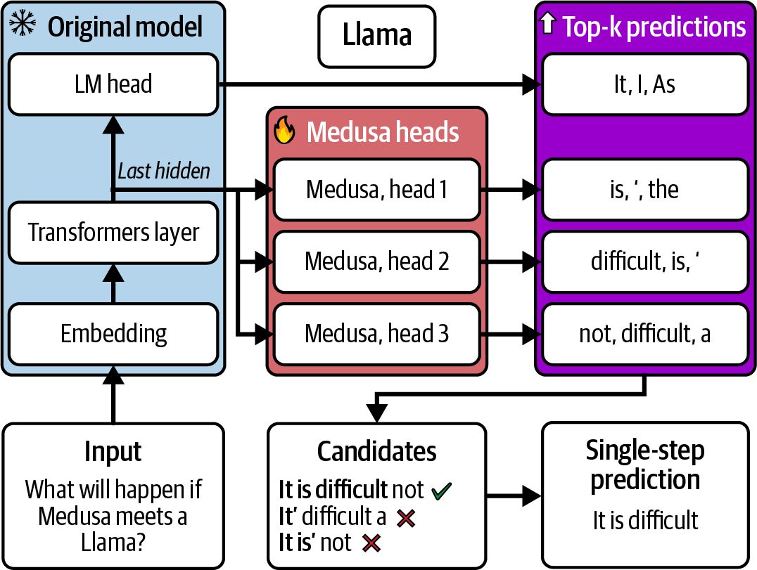
Multitoken Decoding with Medusa’s Multiple Heads Speculative decoding still ultimately generates tokens one by one using the draft model—it’s just faster because the draft model is smaller. However, the Medusa framework takes a more radical approach. It modifies the model architecture itself to predict multiple new tokens in parallel for each decoding step. Unlike two-model speculative decoding, which still generates tokens one by one (albeit faster), Medusa’s architecture truly generates multiple tokens per iteration
686 | Chapter 15: Multinode Inference, Parallelism, Decoding, and Routing Optimizations
from a single model. As such, Medusa’s multiheaded approach has reported about 2.2–3.6× speedups in published experiments across both Medusa-1 and Medusa-2. However, Medusa requires custom model training since it modifies the transformerbased LLM with additional decoder heads that branch off at certain layers—hence, the name Medusa. This lets the model propose several next tokens simultaneously. The multiple token candidates generated by the different Medusa heads are struc‐ tured like a tree. For instance, Medusa can generate a binary tree of depth 2 in one pass to produce up to 4 tokens. It can then verify the sequence of multiple tokens in parallel, as shown in Figure 15-10.
Figure 15-10. Multitoken decoding with Medusa (source: https://oreil.ly/MJMOQ)
Internally, Medusa uses a specialized, tree-based attention pattern to improve consis‐ tency among the parallel token predictions. The model learns to extend and verify the multiple-token sequences concurrently. With Medusa, the LLM essentially learns to “think ahead” by a few tokens—and output them all at once. During inference, Medusa can reduce the number of sequential decoding iterations by the factor of the parallel predictions. For instance, if Medusa predicts 4 tokens in one pass, it can reduce the required number of forward passes by up to 4× for depth-2 binary tree outputs. In practice, however, Medusa typically achieves about a 2–3× speedup due to the overhead of occasionally having to backtrack when a prediction branch fails valida‐ tion and needs a partial redo. This is similar to the overhead of speculative decoding
Speculative Decoding and Parallel Token Generation Techniques | 687
verification and rejection. For example, if a Medusa LLM generates 4 tokens per itera‐ tion, a reply of 100 tokens would take only 25 iterations of the model instead of 100. Medusa requires modifying and retraining the model to add these extra heads. In addition, Medusa models are slightly larger in size given the additional head parame‐ ters. This increases development complexity and training cost a bit. However, once trained, Medusa models can significantly reduce inference times. If trained for your use case, a Medusa-enabled LLM can provide excellent low-latency performance. However, this technique requires modifying and fine-tuning the model architecture to add the additional heads.
Interleaving Decode Steps from Multiple Requests Another parallel decoding technique is to interleave decode steps from multiple con‐ current requests across multiple end users. This parallelism is more of an inferenceengine capability than an algorithmic trick or model architecture modification. But it helps keep the GPUs busy by batching at the token level—and across end-user requests. Frameworks like vLLM implement this in the form of request routing, continuous batching, and token scheduling. The idea is to keep the GPUs busy by filling in the gaps between sequential steps. Specifically, if a GPU is stalled due to a sequence wait‐ ing on I/O or a data dependency, the scheduler can run another sequence’s next token prediction on that same GPU in the meantime.
                     Combining an inference engine’s advanced routing, batching, and
                     scheduling capabilities with CUDA streams. Then verify with
                     Nsight Systems that token-step kernels overlap with NIC/NVLink
                     transfers rather than serializing on a single stream. Then you can
                     achieve massive parallelism at the application, system, and hard‐
                     ware levels.
It’s important to note that interleaving decode steps doesn’t speed up a single sequen‐ ce’s latency. In fact, it can even add a tiny bit of overhead per token due to the addi‐ tional context switching. However, it can greatly improve overall throughput and GPU utilization when serving many users concurrently. This will reduce the average end-user request latency under heavy load.
Combining Decoding Techniques and Evaluating Complexity It’s worth noting that these decoding optimizations can be combined. For instance, one could use speculative decoding with a Medusa-enabled target model in which the big target model verifies multiple tokens at a time predicted by a small model.
688 | Chapter 15: Multinode Inference, Parallelism, Decoding, and Routing Optimizations
These techniques also come at the cost of additional complexity. Either you have to maintain an extra model, alter the main model, or manage more elaborate control logic. In production, you should evaluate this complexity against the performance gains. For interactive applications, reducing response time by even a few milliseconds is worth the complexity—especially at scale. In short, advanced decoding techniques like speculative decoding—with or without a draft model—and Medusa-style multitoken prediction can reduce overall inference times of modern autoregressive LLMs that traditionally generate one token at a time. By generating more tokens at a time, increasing overall arithmetic intensity, and pushing the decoding step toward the compute-bound regime, you can take advan‐ tage of the GPU’s extreme compute capabilities.
               The decoding-optimization landscape is continuously evolving and
               growing in complexity; the trend is clear: make LLM decoding
               more parallel and efficient.
Constrained Decoding Performance Implications A separate but important aspect of the LLM decoding process is generating text under certain constraints. For instance, the model can force the output to match a predefined format (JSON), use a particular grammar, or disallow certain sequences for safety. As such, constrained decoding, often called structured outputs, is often required for production use cases. OpenAI’s function-calling API, for example, relies on well-structured output formats to determine which function to call—as well as the functions’ inputs and outputs. These constraints are designed to match the function’s API signature and are simply nonnegotiable at the application level. Constrained decoding alters the model’s token-selection process so that, at each step, only valid tokens are allowed. This might be as simple as supplying a list of allowed tokens—or as sophisticated as embedding a formal grammar and using a state machine to filter out invalid tokens. The drawback of constrained decoding is that extra latency is needed to enforce these constraints—often a few milliseconds per token. This is because the model may need to backtrack repeatedly, navigate the pruned vocabulary, and ultimately generate a valid token. Backtracking happens inside the LLM’s generation loop. As such, debug‐ ging, profiling, and tuning constrained decoding can be difficult without fine-grained telemetry in the model itself.
Constrained Decoding Performance Implications | 689
Another performance consideration is cache efficiency. Pruning the full probability distribution at every decode step can blow caches and reduce throughput even fur‐ ther. This is particularly noticeable when the allowed token set is heavily limited. To mitigate these costs, many frameworks compile a JSON grammar and precompute valid tokens for each state. This allows the inference engine to mask out invalid soft‐ max outputs at runtime. This approach reduces backtracking, improves caching, and raises acceptance rates. For moderate constraints such as simple JSON schemas, modern engines that use compiled grammars and overlap mask computation with GPU execution can push overhead into the low single-digit percent range at scale, but complex grammars or small batches can still incur double-digit overhead. Always measure TTFT and tokens per second under your exact schema. These techniques have been implemented in popular libraries and inference engines, including Hugging Face Transformers, NVIDIA NeMo, and vLLM. For instance, NVIDIA’s TensorRT-LLM and Hugging Face Transformers both allow user-defined vocabulary masks to enforce constraints with negligible speed penalty. Specifically, TensorRT-LLM exposes guided decoding with JSON schema and context-free gram‐ mar (CFG) support through the XGrammar backend. And vLLM and Transformers provide structured output APIs.
                     When using TensorRT-LLM’s guided decoding, XGrammar sup‐
                     plies JSON-schema and CFG support on-GPU. XGrammar com‐
                     piles constraints and avoids large Python-side token-mask
                     overhead. However, be aware that certain configurations may fall
                     back to slower backends and cause excessive first-request stalls. As
                     such, it’s important to keep grammars compact to preserve cache
                     locality and token-mask bandwidth.
Another popular strategy is to push constrained decoding into the kernel itself. In this case, it would inject token masks during the final softmax step to achieve similar performance gains. When implemented efficiently, constrained decoding can often run as fast as uncon‐ strained decoding—especially if the constraint ruleset is not too large or too restric‐ tive. If the decoding constraints are too restrictive, decoding effectively becomes a search through a small token space. This leads to more backtracking and slower token generation.
690 | Chapter 15: Multinode Inference, Parallelism, Decoding, and Routing Optimizations
                When possible, avoid large or overly restrictive constraints, such as
                grammars, formats, and vocabularies. One option is to let the LLM
                decode as normal and simply postprocess or filter the outputs.
                However, this is not always a performant or viable option. Profile
                the different options and choose what’s best for your use case.
Dynamic Routing Strategies for MoE Inference Serving MoE models efficiently requires careful partitioning of experts across GPUs using expert parallelism. In addition, you need an intelligent and dynamic mecha‐ nism, or gating network, to dynamically route tokens to these experts at runtime. During MoE inference, each token’s forward pass must be routed by the gating net‐ work to one or more expert GPUs. The system needs to handle this communication in a balanced way to keep the GPUs busy—and avoid overloaded GPUs, or hotspots. Let’s examine how to address these in a high-scale, multinode inference environment.
Expert Communication Optimization During the all-to-all exchange of token activations across experts, an MoE shuffles a batch of tokens between the GPUs. Each GPU receives only the tokens it needs for the experts that it hosts, as shown in Figure 15-11. This happens for every layer in the MoE and is a costly operation, which can potentially dominate inference time if not handled efficiently.
Figure 15-11. Each GPU receives only the tokens it needs for the expert(s) that it hosts
One strategy to reduce communication overhead is to use a hierarchical routing strat‐ egy for our GPU cluster by first routing tokens between GPUs within the same node using NVSwitch/NVLink (fast) and routing across nodes only for any remaining tokens that need nonlocal experts. This two-stage all-to-all can reduce the volume of internode traffic.
Dynamic Routing Strategies for MoE Inference | 691
Additionally, you can use asynchronous communication by overlapping the commu‐ nication with computation. High-performance MoE inference servers use doublebuffer communications so that while one batch of tokens is being sent around, the previous batch’s expert computations occur in parallel. This pipelining hides much of the communication latency.
                     It’s possible to achieve near-optimal all-to-all completion times
                     when the internode fabric is kept fully utilized while intranode
                     shuffles run in the background. Be sure to measure link utilization
                     on both the internode NIC and intranode NVLink paths.
A naive implementation of expert routing that uses a single global all-to-all barrier can leave GPUs waiting on synchronization overhead. This wastes bandwidth if not all links are utilized optimally. Techniques such as a butterfly schedule (aka shifted all-to-all schedule) can break the communication into phased rounds. This way, every NVLink/NIC is busy with par‐ tial exchanges—as opposed to one big synchronization. This staggered approach improves link utilization and reduces idle time. All-to-all exchanges may use the built-in ncclAllToAll collective or grouped send and receive calls. Throughput often improves when the exchange is chunked and pipelined or when a hierarchical schedule such as butterfly is used across nodes. Vali‐ date and choose the algorithm that matches your topology.
                     Keep first-stage all-to-all intra-rack (NVLink) and spill inter-rack
                     only for residual tokens. Profile link utilization to confirm NICs
                     are saturated while NVLink shuffles run in the background. Also,
                     when internode links are the bottleneck, it’s recommended to
                     double-buffer MoE all-to-all communication with expert computa‐
                     tion. You can use chunked/pipelined exchanges and butterfly/shif‐
                     ted schedules to avoid global barrier slowdowns and outperform
                     float global collectives.
Another solution to reduce communication traffic is called expert collocation. The idea is to collocate certain experts together on the same GPU or node to avoid unnec‐ essary communication. Consider two experts, experts 5 and 7, that are often activated for the same token by the token router. Placing experts 5 and 7 on the same GPU can eliminate an extra all-to-all hop. Profiling tools and gating-frequency analysis can help identify such pairings for your workload. And yet another solution is to compress the communication between experts, includ‐ ing expert-exchange activations. For instance, you can cast to FP8 or NVFP4 on Ten‐ sor Cores with the NVIDIA Transformer Engine before performing an all-to-all
692 | Chapter 15: Multinode Inference, Parallelism, Decoding, and Routing Optimizations
communication. This will reduce NIC load which amortizes the compression compu‐ tation. This trades a tiny bit of numerical precision for faster activation transfers between GPUs. The overhead to cast and pack/unpack is usually small relative to net‐ work and memory transfer costs. In short, optimizing MoE communication involves analyzing the hardware and net‐ work topology to optimize the placement of experts onto GPUs. For your deploy‐ ments, it’s important to configure the cluster’s interconnects for efficient all-to-all communication. For instance, use the NVLink Switch mesh in an NVL72 rack to get the full bandwidth communication between up to 72 GPUs in a single domain. Naive all-to-all choices can dominate layer time and achieve very low SM efficiency. Priori‐ tize expert traffic and overlap where possible, and make sure to profile and verify when making different interconnect and communication-algorithm choices.
               For MoEs, configure your cluster to optimize for all-to-all commu‐
               nication. This means selecting the appropriate NCCL all-to-all
               algorithm or grouped send and receive implementation for your
               topology, then confirming GPUDirect RDMA is enabled for the
               internode paths. Also, make sure your InfiniBand links are prop‐
               erly bonded such that multiple physical links (ports) are configured
               as a single logical channel. Their bandwidth should be combined—
               and failover should be seamless. In other words, make sure your
               network topology is tuned for MoEs. This includes both the hard‐
               ware and software layers in the stack.
Load Balancing, Capacity Factor, and Expert Replication It’s recommended that each expert and GPU get an equal share of the work to avoid “hotspots.” Otherwise, if the MoE’s gating network directs a disproportionate number of tokens to a particular expert, those GPUs will become overloaded. This will increase latency and reduce overall system throughput. Consider a single expert GPU that becomes a hotspot with utilization hitting 99% while the other expert GPUs are averaging around 60% utilization. This can bottle‐ neck an entire training or inference cluster if not properly handled. During model training, hotspots can be addressed by adding a load-balancing loss term that penalizes the gate if it overuses some experts and underuses others. The result is that the trained MoE model tends to distribute tokens fairly evenly across the experts. At inference time, however, specific input prompts or topics might still cause imbal‐ ance by concentrating on a subset of “hot” experts. One strategy to avoid inference hot spots is to use a capacity factor that triggers an overflow mechanism.
Dynamic Routing Strategies for MoE Inference | 693
By specifying a capacity factor, the model can be configured such that each expert can process only a maximum number of tokens (e.g., 32 tokens) at a given time. If an expert receives more than this capacity of tokens, the extra tokens can either be for‐ warded to a fallback expert with the next highest routing score or the tokens will be serialized and processed in a second pass. Figure 15-12 compares a capacity factor of 1.0 versus 1.5.
Figure 15-12. Comparing expert capacity factors of 1.0 versus 1.5
In practice, a capacity factor of 1.2 (20% overflow allowance) with top-2 gating is common. This means that each expert will take up to 120% of its average load. After that, it will send excess tokens to the next expert. This will effectively smooth out the load across experts in the system. Another strategy to avoid hotspots is expert replication. If one expert is consistently a hotspot, the system can clone that expert onto another GPU. This way, the gating function can send some fraction of tokens to the expert clone running on the other GPU. The replicas are a pure application-level optimization implemented by the inference engine. The model itself is not aware of the replicas. Because replicas are registered as separate experts with their own indices—and often on different GPUs—the engine can route tokens across both the original experts and their clones according to their relative routing scores.
694 | Chapter 15: Multinode Inference, Parallelism, Decoding, and Routing Optimizations
               Replicating experts will increase the memory—and cost—of each
               replicated expert. But since only a few experts tend to be overloa‐
               ded, replicating a small number of hot experts is a targeted fix—
               and won’t double the cost by replicating a full model and all of its
               experts.
Also, replication requires careful handling to keep the replicas synchronized if the model is updated. It’s important that all replica experts remain identical (e.g., same weights) since the gating router knows about only a single expert and does not actually know about the replicas.
               Typically, replicas are loaded from the same checkpoint as the orig‐
               inal model—and not updated independently. This prevents diver‐
               gence between the original expert and its replica.
Adaptive Expert Routing and Real-Time Monitoring Unlike traditional MoE expert gating, which is fixed after training, adaptive routing can adjust the gate’s decisions in real time during inference to react to current condi‐ tions and expert load. For instance, if the system detects that one expert GPU is lag‐ ging behind, it could instruct the gating function to divert some tokens to another expert. The other expert might have a slightly lower routing score, but it receives the request because it has available capacity. You should implement continuous monitoring of per-expert utilization and response latency metrics. Modern MoE systems integrate with telemetry frameworks such that each expert emits utilization metrics to Prometheus/Grafana. This way, the system can dynamically adjust the capacity factor or gating algorithm on the fly. Most LLM expert gating functions only consider routing scores determined at train‐ ing time. However, a truly adaptive system needs to be handled by the inference engine and performed dynamically at inference time. To implement adaptive routing, the inference engine needs to wrap the model’s for‐ ward pass in custom logic. For example, it can intercept the gating softmax and real‐ locate some tokens to different experts based on current load metrics. Inference engines rely on real-time metrics like per-GPU utilization and per-expert token counts to continuously measure expert load. If the system sees one expert’s GPU at 99% utilization while other experts’ GPUs are at 60%, the system could tem‐ porarily lower its load by routing some tokens to its expert replica—or to a different expert with a slightly lower expert-preference score.
Dynamic Routing Strategies for MoE Inference | 695
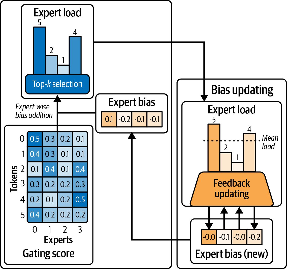
Figure 15-13 shows an adaptive MoE routing strategy that uses a biased gating score approach. While this approach was originally used in a training context, a simpler approach applies to inference. In this case, it would use a modified expert-bias algo‐ rithm to divert tokens to alternate experts when the primary experts are heavily loaded.
Figure 15-13. Adaptive MoE routing in action
This approach can reduce unnecessary communication and balance the load more uniformly. However, it does incur some additional cost in the form of extra monitor‐ ing, decision making, complexity, configuration management, and logging. The bene‐ fits may or may not outweigh the cost. Every scenario and workload is unique, but it’s definitely something worth exploring. When profiling with tools like Nsight Systems, you want to monitor the timeline traces of the expert GPUs’ all-to-all communications. If one GPU’s segment in the timeline is much longer, for instance, it is likely processing more tokens. Your inference system can use these insights to adjust the expert gating probabilities and dynamically reassign experts to different GPUs. It can also spawn additional expert replica instances, etc. This helps to rebalance the load by adjusting the expert gating algorithm, modifying expert placement, or creating/removing expert replicas.
696 | Chapter 15: Multinode Inference, Parallelism, Decoding, and Routing Optimizations
               Dynamically spawning new expert replicas at inference time is
               nontrivial. This approach requires pre-provisioned capacity or
               rapid model loading for those experts. This is an advanced optimi‐
               zation technique.”
Grouping certain experts differently across GPUs can lead to more uniform token routing and increased overall throughput due to better parallelism. This is because the GPUs can finish each layer’s work more synchronously. If persistent imbalance is detected, modern MoE schedulers can dispatch additional expert replicas on the fly by adjusting the capacity factor. This can mitigate a hotspot caused by uneven gating.
               Remember to log any dynamic changes that the system makes. It’s
               also recommended to set up alerts for when a particular expert’s
               utilization goes above a threshold, such as 80% utilization.
Dynamic routing strategies target two core objectives: reduce routing overhead and evenly distribute work across expert GPUs. Achieving low overhead depends on uti‐ lizing high-bandwidth interconnects, overlapping data transfers with computation, and minimizing redundant data movement with co-location and intelligent scheduling. Load balancing is achieved using simple top-1 or top-2 gating or more advanced capacity-aware gates. It can also be achieved using dynamic replication and expert reassignment. Using a combination of these techniques is common to keep the GPUs busy with maximum computations and minimal communication delays. As long as routing overhead is minimized and the load is balanced, adaptive MoE inference systems can achieve near-linear throughput scaling as you increase the number of experts. For example, doubling GPUs can nearly double your inference throughput. In short, these adaptive export routing and load-balancing optimizations can be inte‐ grated with the parallelism and decoding techniques covered earlier. This way, you can tune your MoE inference system for high performance at ultrascale. Continuous profiling and adaptive algorithms can keep your GPUs busy with computations and avoid idling on communication delays.
               Advanced inference engines can dynamically bypass certain expert
               computations, turn off underutilized experts, or use caching to skip
               experts for certain tokens. This further reduces latency. These tech‐
               niques build on the concepts described in this chapter.
Dynamic Routing Strategies for MoE Inference | 697
Key Takeaways
Serving massive LLMs to billions of end users requires optimizations at every stage of
the inference pipeline. The following are some key takeaways from this chapter:
Disaggregate to optimize both latency and throughput
    Splitting the prompt prefill and decode stages onto separate GPU pools elimi‐
    nates interference. This lets you achieve low time-to-first-token and high tokens-
    per-second simultaneously, instead of trading one for the other. It’s a
    foundational technique for large-scale LLM serving.
Use hybrid parallelism for massive models
    No single parallelism strategy is sufficient for multi-trillion-parameter models.
    Combine tensor, pipeline, expert, and data parallelism as needed. For example,
    shard layers across GPUs (TP/PP) to fit the model in memory, use expert paral‐
    lelism for MoE layers to scale model capacity, and add data-parallel replicas to
    meet throughput demands. The optimal mix is hardware-dependent. Always
    profile and tune your configuration for your workload.
Mitigate sequential decoding bottlenecks
    Advanced decoding methods can greatly accelerate generation. Two-model spec‐
    ulative decoding with a fast draft model often delivers about a 2–3× speedup
    when acceptance rates are tuned for the task. EAGLE-2 reports up to 3.5×
    speedup (20%–40% more than EAGLE-1) on some tasks while preserving the
    target distribution. Medusa implementations report up to 3.6× speedup over
    nonspeculative decoding when trained and validated for the target workload.
    These techniques increase token-level parallelism and arithmetic intensity while
    preserving the large model’s output distribution under standard verification.
    Overall, the result is faster responses without retraining the main model’s output.
    This shows that speculative decoding is a quality-preserving technique.
Maintain output quality and format with constraints
   In production, you often need the LLM to follow strict formats or avoid certain
   tokens. Constrained-decoding techniques let you enforce rules—like JSON sche‐
   mas and banned words—during generation. They add some overhead per token,
   but with compiled grammars and optimized mask paths, constrained decoding
   can often run within a low single-digit percent of normal decoding at scale,
   though complex grammars or small batches may incur higher overhead. Always
   test the performance impact of your constraints. Avoid extremely strict rules, if
   possible. They can slow down generation by causing excessive backtracking.
Balance MoE workloads to scale effectively
    Mixture-of-experts models offer almost linear scaling of model size versus GPU/
    expert count—but only if you handle routing efficiently. Use high-bandwidth
    interconnects and hierarchical all-to-all communication to reduce network
698 | Chapter 15: Multinode Inference, Parallelism, Decoding, and Routing Optimizations
    bottlenecks. Ensure each expert gets a similar amount of work by applying
    capacity limits and top-2 gating to avoid straggler experts. Replicate any consis‐
    tently hot experts to split their load. A well-tuned MoE inference system can
    approach near-linear throughput scaling as you add GPUs.
Leverage hardware-software codesign
    Modern GPU hardware is built to support these parallel and distributed infer‐
    ence methods. Use software that takes full advantage of the hardware and topol‐
    ogy, including inference engines like vLLM, SGLang, and NVIDIA Dynamo.
    These can orchestrate multi-GPU and multinode inference with minimal over‐
    head. Align your strategy with your hardware’s strengths by keeping intranode
    communication on NVSwitch, using InfiniBand only when necessary, and over‐
    lapping communications with computations. This alignment is key to achieving
    the best latency and cost-efficiency.
Understand complexity versus return on investment (ROI)
   Each optimization adds system complexity. Techniques like speculative decoding
   and adaptive MoE routing can significantly improve performance, but they
   require extra models or intricate logic. Always weigh the cost. For interactive
   applications, a 2–3× latency improvement is usually worth it. For simpler use
   cases, a straightforward approach might suffice. Start with the biggest bottle‐
   necks, such as eliminating prefill/decode interference. Then incrementally add
   complexity if needed. Monitor and profile to determine which optimizations give
   the best return on investment.
Conclusion By bringing together disaggregated prefill/decode pipelines, multitoken speculative decoding, dynamic expert routing, and adaptive orchestration, it’s possible to serve LLMs in real time with minimal resource contention and ultra-low latency. Modern inference-serving platforms like vLLM, SGLang, and NVIDIA Dynamo embrace many of these optimizations. They efficiently allocate cluster resources, coordinate the KV cache across nodes, implement speculative and constrained decoding, schedule prefill/decode tasks, and much more. The key is an end-to-end, adaptable architecture that matches algorithmic innova‐ tions with high-performance hardware capabilities. Over the next few chapters, we’ll dive deeper into model inference performance optimizations, including dynamic, adaptive, and multinode serving strategies. We’ll cover everything from application-level prefix caching, latency-aware request routing, and reinforcement-learning (RL)-based cluster tuning to systems-level adaptive memory allocation, precision switching, and congestion-aware resource scheduling.
Conclusion | 699