Ch 18 — Advanced Prefill-Decode and KV Cache Tuning
This chapter builds upon Chapter 17 and dives deeper into advanced optimizations for the inference prefill and decode phases. We’ll build upon the high-level scaling strategies and cover low-level techniques, including single decode “mega kernels,” intelligent KV cache tuning and sharing across GPUs, fast GPU-to-GPU transfer of the prompt state, adaptive resource scheduling, and dynamic routing between prefill and decode workers. We will also highlight hardware and software innovations, which provide new levels of performance and efficiency. By applying these techniques, you can significantly reduce decode latency, improve throughput per GPU, and meet strict latency SLOs at scale.
Optimized Decode Kernels Until now, we have been focused on high-level system and cluster optimization strategies. Another set of techniques to consider when increasing ultrascale inference is low-level kernel and memory management tuning—especially for the decode phase. The decode phase is distributed and often memory bound. This has motivated researchers and practitioners to make the decode phase as fast as possible—and tuned for specific hardware. Two notable innovations in this space are FlashMLA (Deep‐ Seek), ThunderMLA (Stanford), and FlexDecoding (PyTorch). These specifically tar‐ get the transformer’s multihead attention efficiency during decode in variablesequence scenarios common in LLM workloads. Let’s cover each of these next.
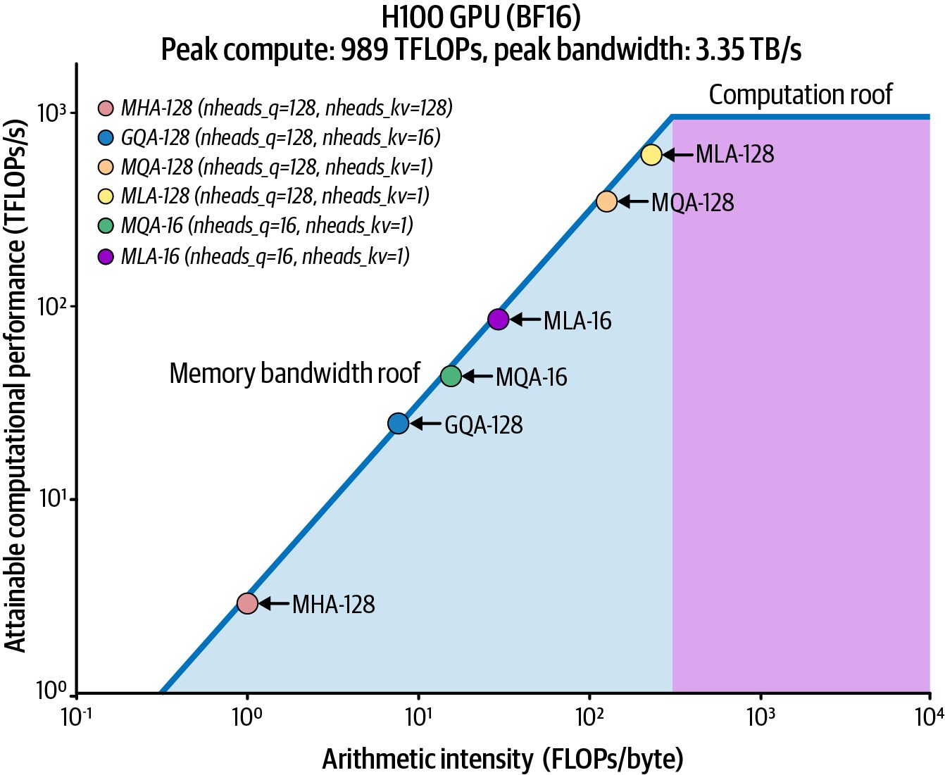
FlashMLA (DeepSeek) Flash Multi-Latent Attention, or FlashMLA, is an optimized decoding kernel intro‐ duced by DeepSeek. It specifically focuses on the single-token decode step, which is essentially the forward pass of a transformer layer used to generate the next token. FlashMLA makes decode faster by fusing operations and better using the GPU mem‐ ory hierarchy. FlashMLA (decode) is to inference what FlashAttention (prefill) is to training. It reduces memory access overhead and latency. With FlashMLA, you can achieve large latency reductions for the decode phase compared to standard kernels. FlashMLA increases arithmetic intensity by fusing multiple attention operations into one. This way, it can process multiple heads and multiple time steps in one fused kernel launch. This increases GPU utilization during the decode by keeping the math units busy despite small batch sizes. Figure 18-1 shows the improvement in arithmetic inten‐ sity for MLA compared to other attention implementations like grouped-query atten‐ tion (GQA) and multiquery attention (MQA) on a Hopper H100 GPU. (Note: Blackwell shifts both rooflines upward with higher TFLOPs and HBM bandwidth.)
Figure 18-1. MLA approaches the compute-bound regime (measured on the NVIDIA Hopper H100 architecture)
800 | Chapter 18: Advanced Prefill-Decode and KV Cache Tuning
The introduction of FlashMLA was significant because it showed that the decode phase’s bottlenecks, memory bandwidth, and kernel-launch overhead can be reduced—even on suboptimal GPU hardware. It reduced the number of separate GPU kernel launches and optimized memory access patterns—squeezing as much performance out of constrained hardware as possible for decoding tasks. DeepSeek’s open sourced FlashMLA implementation is available and seeing adoption. SGLang and vLLM both provide first-class support for DeepSeek models. As such, you should evaluate FlashMLA to increase per-token decode throughput without changing higher-level architecture. Since DeepSeek’s open sourced FlashMLA is integrated into modern inference serv‐ ing systems, you should explore it as a way to increase the throughput of each decode worker—or reduce latency per token—without any higher-level architectural change.
ThunderMLA (Stanford) Building on FlashMLA, researchers at Stanford introduced ThunderMLA, a com‐ pletely fused attention decode “megakernel” that focuses on decoding and scheduling (rather than fusing the full feed-forward block.) This “megakernel” reduces launch overhead and tail effects by combining multiple kernel launches into one—as well as consolidating intermediate memory writes. ThunderMLA reports 20–35% faster decode throughput compared to FlashMLA across different workloads The key idea of ThunderMLA is that when decoding sequences of different lengths, using fine-grained scheduling and fused operations can avoid the tail effect in which some sequences finish earlier while others leave the GPU partially idle. ThunderMLA keeps the GPU busy even if some decode streams complete earlier. It does this by dynamically packing and processing the remaining streams using its fused approach. These benefits are amplified on modern GPUs with larger L2 caches and faster atten‐ tion primitives. Notably, modern NVIDIA GPUs also provide Transformer Engine support for FP8 and FP4 (and FP6, although we focus mostly on FP8/FP4 formats in this text since FP6 is not widely used in existing AI frameworks and tools). Combined with higher memory bandwidth, the Tensor Cores let kernels like ThunderMLA operate much closer to hardware limits. On modern GPUs, ThunderMLA achieves even lower latency per token due to these architectural advances.
Optimized Decode Kernels | 801
FlexDecoding (PyTorch) In Chapter 14, we discussed PyTorch’s FlexAttention, which lets you JIT-compile fused kernels for arbitrary sparsity patterns in attention, including local windows, block-sparse patterns, etc.—all without writing custom CUDA. Under the hood, TorchInductor + OpenAI’s Triton generate a fused kernel that computes only the allowed query-key pairs for that pattern. Triton automatically applies performance optimization techniques like warp specialization and asynchronous copies when ben‐ eficial on the given hardware. However, you can also tune triton.Config to further customize by configuring num_consumer_groups for example. FlexDecoding is the decoding backend of torch.nn.attention.flex_attention. FlexDecoding also lets you manage KV in place and supports masks and biases just like FlexAttention. Specifically, FlexDecoding compiles a specialized kernel for the decode phase (Q_len=1) attending over a growing KV cache. At runtime, the FlexDecoding implementation picks the specialized decode kernel and reuses it across multiple decode steps. This helps to minimize overhead when shapes and dtypes remain compatible—greatly speeding up long-sequence LLM inference.
                    Prefer torch.compile(mode="max-autotune") for stable, latency-
                    critical decode once recompilations are under control. Keep the
                    capture boundary narrow (per-layer or attention block) to reduce
                    graph invalidations from ragged batching. Prefer Transformer
                    Engine FP8 (MXFP8) for prefill and decode. Consider FP4
                    (NVFP4) when accuracy permits and performance increases. As of
                    this writing, FP4 support is still maturing and can underperform 8-
                    bit and 16-bit formats in the near-term. Continue to set
                    torch.set_float32_matmul_precision("high") to enable TF32
                    fallback on remaining FP32 ops. FlexAttention’s decode backend
                    supports common performance enhancements including grouped-
                    query attention (GQA) and PagedAttention.
A key feature of FlexAttention and FlexDecoding includes support for nested jaggedlayout tensors (NJT). These allow ragged batching of variable-length sequences (com‐ mon in LLM workloads) during decoding. A jagged tensor representation of various sequences is shown in Figure 18-2.
802 | Chapter 18: Advanced Prefill-Decode and KV Cache Tuning
Figure 18-2. Ragged batch as a nested jagged tensor (offsets); three sequences (top) repre‐ sented as a single nested jagged tensor representation with offsets (bottom); prefer PyTorch NJT for decode-time batching
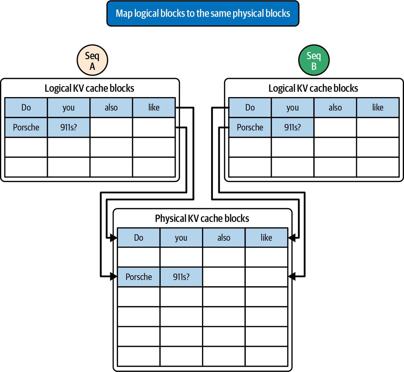
Additionally, FlexDecoding supports bias terms and integrates with PagedAttention by using a block mask conversion interface that maps logical blocks to the physical cache layout. This scatters logical KV blocks into the physical cache layout—without creating extra copies, as shown in Figure 18-3. FlexDecoding leverages captured tensors to vary certain mask or bias values during each iteration—without requiring a recompile. And it integrates with PagedAttention. To use a global KV cache such as vLLM LMCache, map the cache’s page table to Flex‐ Attention’s BlockMask. This will translate logical KV pages into physical memory addresses on the fly. With FlexDecoding, developers have full Python-level flexibility for custom attention sparsity patterns. This is particularly useful for MoE model inference. FlexDecoding allows you to achieve near-optimal performance without requiring you to write any custom CUDA kernels. Essentially, it allows arbitrary attention patterns to be opti‐ mized similarly to dense attention patterns. This becomes even more valuable as new inference techniques emerge.
Optimized Decode Kernels | 803
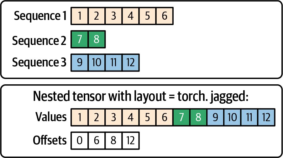
Figure 18-3. PagedAttention scatters logical KV blocks into physical KV blocks for opti‐ mal cache reuse between sequences; align block sizes with LMCache page size—larger pages (e.g., 64–128 tokens) reduce RDMA overhead in disaggregated setups
Many of these capabilities, such as fused attention for decoding and support for PyTorch’s nested jagged tensors (NJT) batching, are available in the core PyTorch library. This makes custom fusion less necessary for typical patterns.
                    Prefer the NJT layout when batching ragged sequences common in
                    LLM workloads.
804 | Chapter 18: Advanced Prefill-Decode and KV Cache Tuning
These kernel-level advancements are highly technical and leverage the full power of the GPU, network, and memory. These software optimizations can significantly improve decode performance—even on the same hardware. When designing an ultrascale system, you should incorporate these optimized kernels, if possible. Be sure to verify overlap and kernel efficiency using Nsight Systems with hardware-based CUDA traces. Additionally, use Nsight Compute for specific memory and link metrics.
               Enabling some of these advanced kernels might require installing a
               custom library or enabling a specialized CUDA kernel—especially
               for newer techniques. However, these techniques are typically sup‐
               ported by PyTorch and the popular inference engines soon after
               they are released. Even if you do need to install custom resources,
               the effort is worthwhile since it will directly translate to lower
               latency and fewer GPUs in the decode worker pool.
Tuning KV Cache Utilization and Management Disaggregation requires that you treat the KV cache as a first-class shared resource across the cluster. Since KV caches can now live longer and move between nodes, high-performance inference systems have improved how the KV cache is stored and shared. In particular, distributed KV cache pools and prefix reuse across requests become powerful techniques. Additionally, it’s important to keep an eye on the memory band‐ width improvements with newer GPU and HBM generations. Let’s discuss each of these in the context of improving KV cache performance.
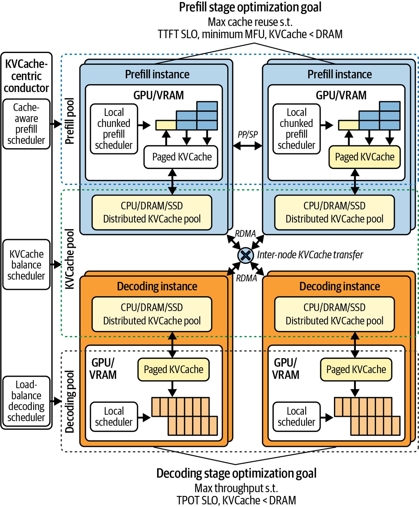
Disaggregated KV Cache Pool Instead of each GPU storing KV only for the requests it’s currently serving, a disag‐ gregated KV cache pool decouples KV storage from individual GPUs. Instead, it spreads the data out across the entire cluster’s GPU memory. The pool can also offload to CPU memory, including the unified CPU and GPU memory of the Grace Blackwell and Vera Rubin platforms. It can also offload to per‐ sistent storage like NVMe SSDs. Using a disaggregated KV cache pool, when a prefill computes the KV tensors for a prompt—or when a decode extends the KV tensors—the KV blocks are stored in a distributed manner across many compute nodes. This is shown in Figure 18-4, adap‐ ted from work on disaggregated KV pools.
Tuning KV Cache Utilization and Management | 805
Figure 18-4. Disaggregated (distributed) KV cache pool (source: https://oreil.ly/2xtK-)
Consider a very long 250,000-token context (e.g., a chat session with many turns) using a 70 billion-parameter transformer model with 80 layers and 32 heads in which each head is dimension 128. This generates a huge KV cache footprint per token. Each token generates a key and value vector of length equal to the model’s hidden dimension (num_heads × head_dim). Let’s assume this is 4,096 for our model. This
806 | Chapter 18: Advanced Prefill-Decode and KV Cache Tuning
results in 8,192 floats per layer. Summing across 80 layers, this creates 655,360 floats of KV data per token. Let’s assume 16-bit precision, or 2 bytes per float. This is roughly 1.31 MB needed per token. Scaling this to 250,000 tokens produces about 328 GB—just for the KV data!
                These calculations are based on per-token KV sizes for large mod‐
                els. This shows why FP8 KV caches are widely adopted in engines
                such as vLLM to reduce footprint and increase batching
                opportunities.
Assuming we quantize the KV cache down to FP8 and use techniques like selectivelayer caching, we can reduce this footprint down to maybe the 100–150 GB range for this 250,000-token prompt. A single GPU will likely not have capacity for all of the tokens’ KV along with everything else it needs to hold, such as model weights, etc.— especially as the multiturn conversation continues. As such, the system would need to truncate context—or cause expensive KV recomputation on earlier tokens. With a disaggregated KV pool, however, older parts of the context’s KV can be evicted from the GPU and pushed out to the KV cache pool spread across the cluster—and in CPU DRAM or NVMe storage. The data is then fetched back into GPU memory when it’s needed. A disaggregated KV cache pool implements a multitier memory hierarchy in which GPU device memory holds the active KV cache while the CPU host RAM (or NVMe storage) serves as the overflow backing store. Modern inference engines can choose to offload KV cache to CPU memory or NVMe. This effectively virtualizes GPU memory much like an OS’s virtual memory subsystem. This design allows for ultralong contexts by asynchronously paging KV blocks between GPU memory and the KV cache pool without stalling the compute pipelines—assuming good communication-computation overlap, as discussed throughout this book. Additionally, by decoupling request state from individual GPUs, the system can use the global KV cache pool to dynamically shard KV data across multiple nodes in the cluster to adaptively balance the load. This simplifies scaling and improves fault isola‐ tion in large inference clusters. And since any decode node can access the global KV pool, then any decode node can participate in decoding any request, if needed due to failover or load balancing. This adds flexibility for the scheduler since it can choose a decode node closest to where the relevant KV cache blocks are located.
Tuning KV Cache Utilization and Management | 807
If some KV blocks of a prefix are cached in DRAM on server A, it might be faster to schedule the decode on server A since it can quickly pull them into its GPU. This is in contrast to server B, which would have to fetch the KV blocks over the network.
                    This describes a classic distributed-systems best practice of choos‐
                    ing a compute node that is closest to the data being computed. This
                    way, the system minimizes expensive data movement.
An efficient KV cache scheduler can look at the distribution of KV blocks in the pool—in addition to the network topology—and assign prefill and decode tasks accordingly. As such, a prefill node can place KV data into a pool implemented as a distributed memory space accessible across the cluster. With the KV cache in a cluster-side shared-memory space, any decode node can retrieve the data. This avoids having to schedule for direct prefill-to-decode transfers every time. This adds a bit of extra overhead due to an extra hop to retrieve KV data from the pool, but it allows more flexibility because all decode nodes have access to all KVcached data. It also means that a decode node that didn’t directly receive data from a particular prefill can still access the KV data from the pool, if needed. If a decode node crashes—or a request needs to move mid-generation for whatever reason—the KV data isn’t lost. The data lives in the pool, and another node can pick it up and continue where it left off using the saved KV. This improves fault tolerance. A global KV cache pool also provides cache persistence across requests. This way, if two requests share some prefix, the KV for that prefix can be computed once and reused across the cluster—even if the requests end up on different decode servers. In short, a disaggregated KV cache pool trades memory (or colder storage) for com‐ pute. By storing a larger KV cache, the system can avoid recomputing KV data in many scenarios. This approach leverages the fact that reusing data—even from DRAM or SSD—is often cheaper than repeatedly recomputing large attention matrix multiplications with quadratic time complexity, O(N2).
KV Cache Reuse and Prefix Sharing As mentioned, it’s beneficial to reuse cached KV data across requests for prompts that share a common prefix. This scenario arises fairly often in the form of multiturn con‐ versations, shared system prompts, and attached documents. Instead of recomputing the transformer attention outputs for that prefix for every request, the system can store the KV outputs for the prefix and reuse them directly.
808 | Chapter 18: Advanced Prefill-Decode and KV Cache Tuning
Essentially, this skips the prefill computation for that portion of the input, which saves a lot of time and GPU cycles. A proper KV-cache-centric scheduler takes into account prefix cache hits by looking at the “prefix cache hit length,” or how many tokens of this prompt are already present in the cache pool, when assigning work. In practice, if a new request comes and its first N tokens match some cached prefix in the KV pool, the system can decide to reuse that KV data. vLLM implements automatic prefix caching using a global hash table of KV “pages” using its PagedAttention mechanism. Here, each unique 16-token block of context has a hash. If a new request needs a prefix that matches a stored block (by hash), it can directly copy those KV tensors instead of recomputing. If the same context appears again, the system serves it from memory. In essence, it treats the KV of a context as reusable data that can be looked up by content using hashing. Implementations typically maintain a global “prompt tree” to manage these cached contexts and evict them when necessary. This optimizes for the most fre‐ quently reused prefixes. A key to effective KV reuse is identifying identical or overlapping prefixes. Usually, systems focus on exact matches for simplicity such that if the first N tokens match exactly, they reuse that chunk. Combining partial-prefix overlaps is more complex since you need to somehow merge caches, which isn’t always straightforward. So typi‐ cal caching uses exact prefix caching. There is a trade-off, however. Storing many users’ KV caches indefinitely can con‐ sume a lot of memory. A system must implement eviction policies like LRU for KV blocks to drop caches that are unlikely to be reused. This frees space for new ones. The scheduler might also decide which caches to keep based on likelihood of reuse. The idea is to maximize cache hits within memory constraints. If a certain prefill node already holds a portion of the KV needed in its local GPU memory or local DRAM cache, it might be beneficial to route the request to that node to minimize data transfer. This is an example of data-aware scheduling in which it sends the compute to where the data is, rather than always pulling data to wherever compute is available. This is analogous to locality-aware scheduling in distributed systems. In our earlier routing discussion, we touched on this. If possible, you should route a request to the server that generated its prefix. This maximizes the likelihood of a cache hit. In the broader context of disaggregation, prefix caching is supported by having a uni‐ fied view of KV across many requests and possibly storing it in a shareable place like the global pool. This is in contrast to a siloed per-request or per-node approach.
Tuning KV Cache Utilization and Management | 809
This also helps reduce the overhead of recomputation that disaggregation might otherwise incur if the same prompt goes to different nodes at different times. With a global KV store or coordinated caching, even if a user’s requests hit different decode servers, they can benefit from each other’s cached work.
Optimized KV Cache Memory Layout Another area of low-level innovation is optimizing the KV cache memory layouts. The KV cache, which stores keys and values for all past tokens in each sequence, can become huge for many concurrent decode streams since each stream uses memory roughly proportional to num_layers × 2 × sequence_length × d_head. Techniques like tiered caching are useful since not all KV pairs need to be kept in GPU memory at all times. Older parts of the KV cache can be swapped to CPU—or even compressed. Since we emphasize keeping decode latency low, most designs keep the active KV cache in GPU memory for quick access. In this case, you can tune how the memory is laid out and accessed. DeepSeek’s FlashMLA pages KV cache and allocates the cache in fixed-size blocks (pages) so that contiguous memory accesses can happen for active sequences. This reduces cache misses and DRAM traffic. Additionally, some systems implement prefix compression if a prompt’s prefix will no longer be attended to because the context window has moved, for instance. In this case, the KV cache manager might drop or compress these KV entries. This is more relevant in long conversations because the context window slides. But it can save memory and bandwidth for extremely long sequences.
                    This eviction/compression technique is safe when the model uses a
                    sliding-window or other restricted-attention pattern. However, it
                    should not be applied to layers that retain full attention over the
                    full content window (or retrieval hooks) without careful evaluation.
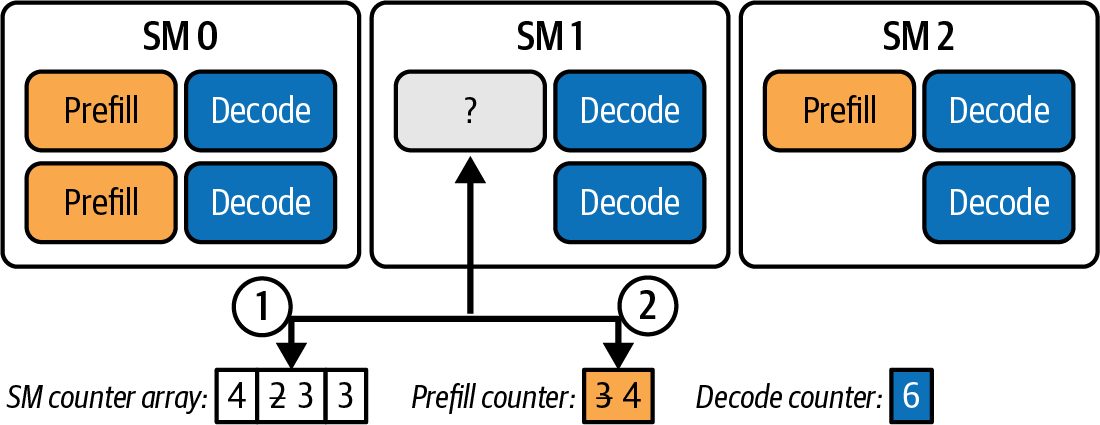
Another technique called POD-Attention similarly reorganizes attention computation to reduce HBM traffic. Specifically, it uses SM-aware thread-block (or cooperative thread array [CTA]) scheduling. This implements runtime operation binding to dynamically assign each CTA running on an SM to either perform a prefill or decode task. This is shown in Figure 18-5.
810 | Chapter 18: Advanced Prefill-Decode and KV Cache Tuning
Figure 18-5. SM-aware thread-block (CTA) scheduling to match prefill tasks with decode tasks on SMs to minimize memory movement
So rather than statically launching separate kernels for each phase, a single kernel launches enough CTAs to cover both workloads. At runtime, each CTA inspects which SM it’s on and uses per-SM counters to decide which operation (prefill or decode) should be run based on what else is running on that SM. The SM-aware scheduling logic tries to match prefill with decode operations at run‐ time. This avoids isolated bursts of memory traffic and smooths out resource demands. Specifically, POD-Attention colocates prefill and decode work on the same SM so the fused kernel can improve locality and reduce redundant HBM transactions. This minimizes memory movement, maximizes bandwidth utilization, and balances compute-bound and memory-bound workloads on each SM. POD-Attention can improve attention performance by up to about 29% by colocating prefill and decode work on the same SMs with proper SM-aware CTA scheduling to unlock full overlap. POD-Attention’s dynamic binding decouples the hardware’s CTA-SM assignment from the software’s CTA-role assignment—either prefill or decode. This type of inno‐ vation shows a growing focus on hardware and software codesign to minimize mem‐ ory movement and get the most out of your system’s performance.
GPU and CPU-GPU Superchip Improvements You should also consider memory bandwidth improvements in new hardware. Higher memory bandwidth and larger L2 caches directly benefit the performance of the memory-bound decode phase. NVIDIA’s Grace Blackwell GB200 NVL72 system, a rack-scale platform with 36 Grace CPUs and 72 Blackwell GPUs, allows a single logical decode unit with tens of tera‐ bytes of memory for KV cache. This hardware, with its ~30 TB of unified memory, is ideal to keep very large contexts in memory. These contexts can be on the order of millions of tokens.
Tuning KV Cache Utilization and Management | 811
With such a platform, the unified memory footprint is large. However, for latencycritical decode, you still want the active keys and values to live in GPU HBM. As such, you should use Grace CPU memory (LPDDR5X, not HBM) as a lower-tier cache or for very old tokens. Prefill and key-value offloading remain important when contexts exceed available HBM—even on a system like the NVL72. In short, disaggregation at a macro level should be paired with microlevel optimiza‐ tions to fully achieve maximum inference performance. Advanced decode kernels like FlashMLA/ThunderMLA, efficient memory layouts (paged caches, etc.), and the latest GPU architectures will produce efficient and scalable decode.
Fast KV Cache Transfer Between Prefill and Decode A key requirement of disaggregated inference is quickly and efficiently transferring the KV cache from the prefill worker to a decode worker. If this transfer isn’t fast, any time saved by parallelizing prefill and decode could be lost waiting on data movement. In this section, we discuss the techniques used to minimize transfer overhead. We then describe how systems implement the handoff, using high-speed interconnects and avoiding extra KV copies.
KV Cache Size Prefill output consists primarily of the KV cache for all prompt tokens. This can be a lot of data. Consider a model with L layers, each with h attention heads of dimension d, and a prompt of N tokens. The KV cache size is roughly 2 × L × N × (h × d), where the factor, 2, is for both keys and values. The actual size depends on precision (FP16 versus INT8, etc.) and model specifics, but it’s large. For instance, a 40-layer model with 16 heads of size 64 and a 1,000token prompt produces on the order of 40,000 KV vectors. This could be hundreds of MB of data. If the number of tokens is 5,000, it’s 5× larger. Transferring this amount of data over a network can introduce significant latency if done naively. For instance, a naive approach might be to copy the KV to CPU mem‐ ory on the prefill worker, then send it over TCP—or even write it to disk for the decode process to load. This could be extremely slow, on the order of hundreds of milliseconds for large prompts. The goal is to reduce the transfer time down to only a few milliseconds. This allows prefill and decode to truly overlap in parallel.
                    Achieving low-latency KV data transfer times typically requires col‐
                    lating small PagedAttention blocks into larger buffers and moving
                    them with GPUDirect RDMA-based paths rather than CPU sockets.
812 | Chapter 18: Advanced Prefill-Decode and KV Cache Tuning
Zero-Copy GPU-to-GPU Transfer Modern disaggregated systems use zero-copy GPU-to-GPU transfer techniques. In practice, this involves using remote direct memory access (RDMA) over high-speed fabrics. For example, you can use InfiniBand for transfer between racks/nodes—or use NVLink/NVSwitch for direct GPU memory writes within a single node (multiGPU) platform. These methods send data directly between GPUs without copying through CPU memory. NVIDIA’s high-performance GPU-to-GPU transfer library for inference is called NVIDIA Inference Xfer Library (NIXL). NIXL provides a plugin architecture (e.g., NVLink, UCX fabrics, GPUDirect Storage) for zero-copy GPU↔GPU and GPU↔storage data movement. NIXL streamlines RDMA-style transfers, allowing one GPU to write directly into another GPU’s memory over the available high-speed fabric—for example, Infini‐ Band or NVLink-based connections. In other words, the prefill GPU can directly inject the KV tensors into the decode worker GPU’s memory. RDMA-based protocols bypass the CPU and make full use of the GPU interconnect bandwidth. Systems like NVIDIA Dynamo and the open source vLLM plus LMCache integration rely on NIXL. Specifically, they use NIXL to write KV tensors directly into remote GPU memory over NVLink or RDMA. Modern GPU interconnects provide very high bandwidth, and a 1 GB transfer can complete in a few to tens of milli‐ seconds depending on link type and contention. In practice, implementations achieve low transfer times by overlapping data transfer with computation. For instance, with RDMA, a decode GPU can continue generating tokens for other sequences while a prefill worker is writing KV data into its memory buffer asynchronously. The prefill can push the data (RDMA write push model), or the decode can pull it (RDMA read), depending on design. Either way, no CPU involvement is needed in the data path. Common strategies for fast KV transfer include prefill-side push, decode-side pull, shared-memory (CUDA IPC) buffer, connector/queue abstraction, and nonblocking overlap. Let’s discuss each of these: Prefill-side push The prefill worker, upon finishing the prompt, initiates an RDMA write of the KV data directly into a reserved buffer on the decode worker’s GPU. This can be done nonblockingly; the prefill can start the transfer and then move on to other work while the DMA occurs in the background.
Fast KV Cache Transfer Between Prefill and Decode | 813
Decode-side pull Alternatively, the decode worker can RDMA-read directly from the prefill GPU’s memory when it’s ready to begin decoding. Either push or pull achieves the same end result (no CPU copies). Some implementations might prefer push to offload coordination to the sender; others prefer pull for the receiver to control timing. Shared-memory (IPC) buffer If prefill and decode happen to be on the same machine (different GPUs in one server), they might use CUDA interprocess communication to share a memory handle or even a PCIe bar, effectively copying using NVLink or NVSwitch on the same host. This is a local variant of zero-copy transfer without going over the network. Connector/queue abstraction vLLM’s implementation abstracts the transfer mechanism behind a logical inter‐ face (a Pipe or LookupBuffer). The prefill process places the KV into this buffer or signals its availability, and the decode side retrieves it. Under the hood, this can use RDMA or even a high-performance pub-sub message (NATS in Dyna‐ mo’s case for control signals). The key is to decouple the logical handoff from the transport so different transports (RDMA, shared memory, etc.) can be plugged in. Nonblocking overlap As mentioned, optimized systems overlap KV transfer with ongoing decode computations. For example, Dynamo’s decode worker continues generating tokens on other requests while a prefill worker is writing KV data into its GPU memory for a new request. This hides much of the transfer latency. As such, you can overlap a ~5 ms KV transfer with decode computation and add virtually zero net latency to the request’s first generated token. With these methods, KV transfers can take on the order of a few milliseconds. This is much less than the hundreds of milliseconds required to actually compute that KV on the prefill worker. As such, the pipeline of prefill → transfer → decode achieves good parallelism since the decode can start almost immediately after prefill completes— without a long stall. Be careful to avoid fragmentation and overhead when sending KV cache data. For instance, vLLM’s PagedAttention stores the KV cache in fixed-size token blocks, com‐ monly 16 tokens per block. The KV blocks are relatively small (although the bytes per block scale with the number of heads, head dimension, number of layers, and dtype.) Naively sending thousands of small KV pages over RDMA would incur excessive overhead since each transfer has fixed latency and protocol overhead. This would lead to poor bandwidth utilization.
814 | Chapter 18: Advanced Prefill-Decode and KV Cache Tuning
                Modern LLM engines support multiple page sizes, such as 8, 16, 32,
                64, or 128 tokens per block. Larger page sizes can reduce transfer
                overhead when moving KV over RDMA because sustained link
                throughput improves with larger collated buffers and fewer work
                queue elements (WQEs). When possible, collate ≥ 128-token pages
                per RDMA write. Make sure to overlap the transfer on a dedicated
                CUDA stream. Prefer nonblocking streams and use event fences.
                Always profile with tools like Nsight Systems to confirm overlap.
                LMCache reports ~20 ms → ~8 ms for a 7.5k-token KV after colla‐
                tion on RDMA.
The LMCache extension addresses this inefficiency by collating KV pages into large
contiguous buffers before transfer. Essentially, it gathers the small chunks into one big
chunk in GPU memory, then sends that large buffer in one transfer.
For instance, if sending a 7,500-token KV cache as 470 small transfers takes 20 ms,
collating them into larger blocks (e.g., 128-token pages) reduces transfer time down
to 8 ms. This simple batching optimization keeps the network pipe full and reduces
per-packet overhead.
Let’s show how a system is configured for fast GPU-to-GPU KV transfer. Here is an
example config for LMCache’s prefill-decode mode using a NIXL transfer channel:
    # Prefill server config (lmcache-prefiller-config.yaml)
    enable_pd: true
    transfer_channel: "nixl"
    pd_role: "sender"              # this instance sends KV data
    pd_proxy_host: "decode-host" # PD proxy / decode coordinator
    pd_proxy_port: 7500            # control-plane port on the proxy/decoder
    # size the buffer to the KV you plan to transfer
    # FP8/FP4 KV should shrink it significantly
    pd_buffer_size: 1073741824     # 1 GiB transfer buffer size
    pd_buffer_device: "cuda"       # buffer stays in GPU memory
Here, the prefill server is configured as the RDMA sender. It targets the decode host’s
port 7500 with a 1 GB GPU buffer allocated for KV transfers. The decode server is
configured as the receiver on that port with a matching 1 GB GPU buffer, as shown
here:
    # Decode server config (lmcache-decoder-config.yaml)
    enable_pd: true
    transfer_channel: "nixl"
    pd_role: "receiver"            # this instance receives KV
    pd_peer_host: "0.0.0.0"        # bind address for NIXL peer
    pd_peer_init_port: 7300        # NIXL handshake/control port
    pd_peer_alloc_port: 7400       # NIXL allocation/data port
    pd_buffer_size: 1073741824     # 1 GiB (match sender unless you plan to shard)
    pd_buffer_device: "cuda"       # keep buffer in GPU memory
    nixl_backends: [UCX]           # UCX backend is sufficient for disagg
Fast KV Cache Transfer Between Prefill and Decode | 815
This configuration allows the prefill to write the KV cache directly into the decode GPU’s memory—up to 1 GB per transfer—with no CPU intervention. Both sides keep the transfer buffer in GPU memory for zero-copy operation. When sizing the transfer buffer, start at pd_buffer_size = 1 GB. This is roughly a FP16 KV cache estimated at ~4–8k tokens for a model with 70-billion parameters, 80 lay‐ ers, 32 heads, and 128-dimension heads. Use 2 GB if prompts exceed ~7.5k tokens. You can scale with the dtype and head count: bytes ≈ 2 × L × N × (H × Dh) × bytes_per_val. Make sure to collate pages before transferring. This will avoid smallIO inefficiency.
                    If you quantize the KV cache to FP8 or FP4, the required transfer
                    buffer for a fixed token count decreases since the number of bytes
                    per token decreases accordingly. As such, you can either transfer
                    more tokens per buffer or reduce the buffer size accordingly. A 1-2
                    GiB buffer works for many deployments, but size it from the KV
                    formula above and round up to a 256 MB boundary. If using FP8
                    or FP4 KV, you can shrink the buffer proportionally. Always vali‐
                    date against the largest collated page group you’ll transfer. Prefer
                    GPUDirect RDMA with collation to ≥ 128-token pages for best
                    link utilization.
In practice, one might launch the decode server with the CLI using the following shell
script. This will reduce eager fragmentation and encourage rendezvous on larger
buffers:
      # Example decode worker
      # (select device by index or UUID)
      UCX_RNDV_THRESH=16384
      UCX_MAX_EAGER_RAILS=1
      UCX_TLS=cuda_ipc,rc,rdmacm,cuda_copy,cuda_ipc,tcp \
      CUDA_VISIBLE_DEVICES=1 \
      LMCACHE_CONFIG_FILE=lmcache-decoder-config.yaml \
      python run_vllm_decoder.py --port 8200
You would similarly start the prefill server on another GPU with its config file. These
settings ensure the system uses InfiniBand RDMA across nodes or NVLink peer-to-
peer within a node rather than standard TCP sockets for KV transfer.
816 | Chapter 18: Advanced Prefill-Decode and KV Cache Tuning
                For single-node, multi-GPU runs, you should enable CUDA IPC.
                When running across nodes, prefer RDMA. A typical UCX config
                for LMCache/vLLM workers is to set UCX_TLS=rc,rdmacm,
                cuda_copy,cuda_ipc,tcp and ensure RoCE/IB lossless settings
                (ECN/PFC) are applied on the fabric. For internode RDMA, con‐
                sider UCX_RNDV_THRESH=16384 so that large KV buffers use
                rendezvous and small KV buffers use eager. Always validate with
                ucx_info -f.
With RDMA and proper buffering in place, the handoff latency can be in the singledigit to tens of milliseconds depending on the interconnect and page size. For exam‐ ple, with a 7,500-token context, LMCache measured about 20 milliseconds with many small transfers and about 8 milliseconds after collating into larger blocks. Specifically, it’s recommended to collate 16-token pages into ≥ 128-token slabs before RDMA. This will help reduce per-packet overhead. In short, disaggregated systems should use fast interconnects and smart data collation to make the prefill → decode transition seamless and fast. Minimizing handoff time is critical because if the handoff is slow, it negates the benefit of parallelizing the phases in the first place.
                Use a deterministic hash for KV-chunk routing in multiprocess
                runs by setting export PYTHONHASHSEED=0.
Connector and Data Path Design Building on the zero-copy optimization, let’s see how the prefill and decode nodes coordinate the transfer end to end—beyond just moving the bits. The prefill and decode workers often communicate using a scheduler or router. In practice, this scheduler is often implemented as a centralized component, as used in NVIDIA Dynamo, or a decentralized coordination approach, as used by SGLang. For instance, NVIDIA Dynamo implements a global scheduling queue in which the decode workers push new prompt tasks into a queue that prefill workers consume. In this design, a decode node enqueues a request for prompt processing, as shown in the “Put RemovePrefillRequest” (step 6) in Figure 18-6.
Connector and Data Path Design | 817
Figure 18-6. Request lifecycle in NVIDIA Dynamo; decode pulls prompts and prefill pushes KV using NIXL
818 | Chapter 18: Advanced Prefill-Decode and KV Cache Tuning
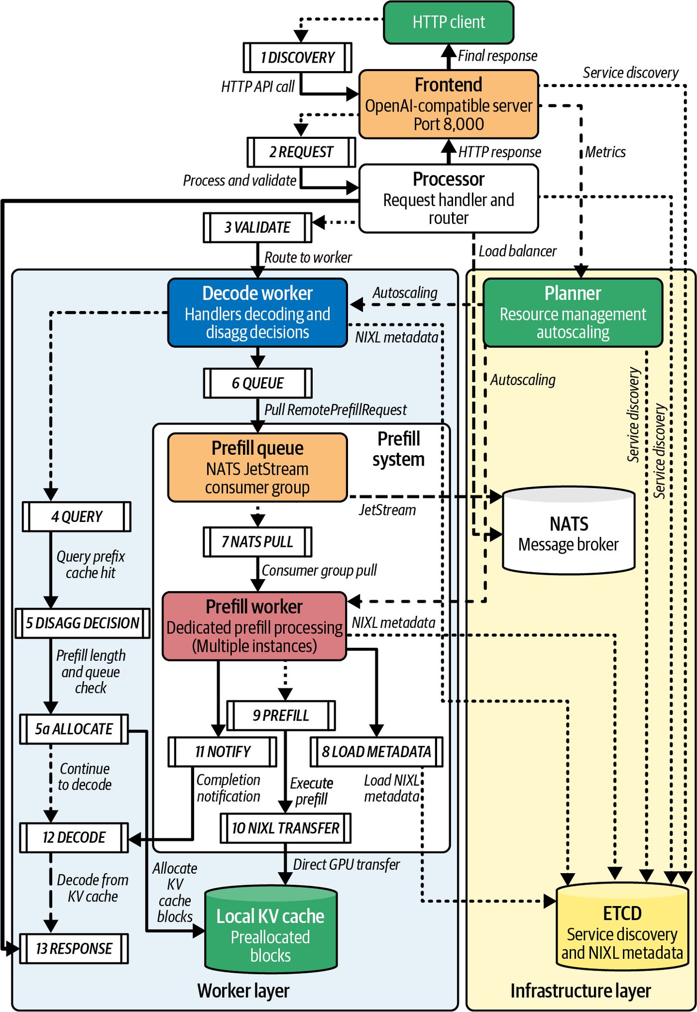
A prefill node picks up this request and, when done, knows exactly which decode node to send the results to since the request carries an origin or reply-to ID for the decode node. The KV is then transferred directly to that decode worker’s GPU using NIXL RDMA. In the vLLM + LMCache implementation, a more decentralized approach is used. The decode and prefill processes establish a direct channel using a pipe or buffer for each request’s KV. Under the hood, this might use a one-to-one TCP or RDMA connection negotiated at request start. Rather than a global queue, each request sets up its own transfer channel. Both approaches have pros and cons. The global queue is simpler for load balancing and failure handling. Direct channels can minimize queuing. When deciding which pattern to use, consider your workload and infrastructure con‐ straints. If you need robust multitenant load balancing and easy failover, and you’re comfortable with a small queuing delay, the global-queue model is usually the better fit. Conversely, if you have stringent tail-latency requirements, a relatively stable set of decode-prefill pairs, and high-speed interconnects, the per-request direct-channel approach can minimize hop count and jitter.
                In practice, benchmark both designs under your anticipated
                request mix. Vary the prompt lengths, concurrency levels, and fail‐
                ure scenarios to see which offers the best latency-throughput trade-
                off for your SLOs.
The key design goal is to make the pipeline nonblocking and high-throughput such that while one request is being decoded, another prompt can start prefilling—mean‐ while, another’s KV can be in transit. As such, no stage sits idle if there is work to do in another stage. This is the exact reason that disaggregation improves overall throughput at scale—all stages are kept busy in parallel.
                Often, the first generated token’s logits from the prefill are often
                not explicitly transferred because the decode worker can simply
                recompute the first token’s probabilities from the KV directly. Some
                systems do transfer the first token’s output to shave off a few hun‐
                dred microseconds of extra compute in the decode worker. But
                other systems keep it simple and just transfer the KV and let the
                decode worker recompute that final layer.
It’s important to make sure that this pipeline is robust to failures. If a decode node fails mid-generation, a global KV cache pool, discussed earlier, can allow another node to pick up where it left off using the saved KV. Similarly, if a prefill node fails midprompt, that prompt can be retried elsewhere. The connector design should handle these failures gracefully so that one node’s failure doesn’t error out the whole request.
Connector and Data Path Design | 819
                    Heartbeat checks and timeouts are commonly used by these rout‐
                    ers so that if a prefill-to-decode transfer stalls, the request can be
                    reassigned or safely aborted.
Heterogeneous Hardware and Parallelism Strategies for Prefill and Decode One powerful advantage of disaggregation is the freedom to choose different hard‐ ware—and even a different model-parallel configuration—that best suits the needs of the prefill and decode clusters separately. In a unified, monolithic deployment, you typ‐ ically have only one hardware type and configuration for both phases. With disaggrega‐ tion, you can mix and match hardware and strategies per phase, as described next.
Compute-Optimized Versus Memory-Optimized Hardware The prefill phase benefits from GPUs with high compute throughput, lots of TFLOPS, specialized Tensor Cores, and high clock rates. It also benefits from sub‐ stantial memory bandwidth, but it doesn’t necessarily require massive HBM capacity beyond what the prompt’s KV cache requires. The decode phase, on the other hand, benefits from both large memory capacity and memory bandwidth since it handles many tokens’ worth of KV. It doesn’t need extreme compute power, but the more the better. This opens up the possibility of using different generations of GPUs for each phase. For example, one design can use the latest high-compute GPUs for the prefill cluster but stick with older-generation or cost-efficient GPUs with sufficient memory band‐ width for the decode cluster. This way, we avoid wasting the newest GPUs (e.g., the latest Tensor Cores) on a task like decode that doesn’t use their full potential. The prefill tasks tend to draw more power by maxing out the GPU math units, whereas the decode tasks use far less power on the same GPU.
Throughput and cost benefits Splitting the phases among heterogeneous hardware can improve throughput per cost and throughput per watt. In the Splitwise study, using phase-specific hardware led to one configuration achieving 1.4× higher throughput at 20% lower cost over a homogeneous baseline. In another configuration aimed at max performance under a fixed cost/power budget, they achieved 2.35× more throughput for the same cost and power. Specifically, this study used 4× H100 (high-compute) for prefill and 4× A100 (high-memory) for
820 | Chapter 18: Advanced Prefill-Decode and KV Cache Tuning
decode. This mixed configuration achieved ~2.35× the RPS of an 8-GPU homogeneous system (either all H100s or all A100s) at the same cost/power. Alternatively, they found that, to match the baseline throughput, the heterogeneous system could actually use fewer GPUs overall (e.g., five or six instead of eight) by off‐ loading decode to cheaper GPUs. This highlights the cost-savings opportunity and shows the value of using each type of GPU where it’s most effective. Specifically, you can perform compute-bound work on the highest-compute-per-dollar GPUs (e.g., Blackwell or Rubin generation) and assign memory-bound work to more cost-efficient older-generation GPUs with suitable memory bandwidth (e.g., Hopper or Ampere). The Splitwise evaluation accounted for the overhead of state transfer between hetero‐ geneous GPUs. This test transferred KV data over an NVSwitch fabric and incurred minimal overhead—even between different generations of GPUs. This indicates that high-bandwidth interconnects like NVSwitch and NVLink can enable prefill/decode disaggregation with negligible impact on performance—even in mixed-GPU setups. Another system is HexGen-2, which is a distributed inference framework that treats the allocation of disaggregated inference on heterogeneous GPUs as an optimization problem. Its scheduler optimizes resource allocation, per-phase parallelism strategy, and communication efficiency together. In experiments on models like Llama 2 70B, HexGen-2 shows up to a 2× improve‐ ment in serving throughput (~1.3× on average) as compared to state-of-the-art sys‐ tems at the same price point. Additionally, it achieves similar throughput to a highend baseline while using approximately 30% less cost. These improvements came from mixing GPU types and optimizing the work split. This is basically an automated way to do what Splitwise did conceptually. These results confirm that disaggregation is not just about speed. It’s also about effi‐ ciency and doing more with less. When deploying inference in a cloud environment, this can lead to significant cost savings on the order of millions of dollars in GPU time for a large inference service supporting millions or billions of end users. For instance, you can fulfill the same traffic with 6 GPUs (prefill + decode mix) instead of 8 top-tier GPUs; you can save roughly 25% on hardware costs for that ser‐ vice. As such, disaggregation lets you serve more users on the same hardware. This is critical since GPU supply is often limited—especially for the latest GPUs. Energy efficiency is also important given power constraints in certain parts of the world, including the United States. Splitwise demonstrated better power efficiency by running decode tasks on lower-power GPUs—at a slight decrease in speed. By assigning prefill and decode tasks onto different hardware types, you can choose where and how to run each phase to increase performance and reduce cost. Disaggre‐ gation allows this flexibility since phases are independent.
Heterogeneous Hardware and Parallelism Strategies for Prefill and Decode | 821
In short, the evaluations from Splitwise, HexGen-2, and related heterogeneous deploy‐ ment studies show that disaggregation can be leveraged for cost optimization in addi‐ tion to pure speed. By matching hardware to workload, you can significantly reduce the cost per query and, at the same time, increase performance within a fixed budget. For large-scale services, this is critical to keep them economically viable. The tradeoffs include a bit more system complexity because you have to manage multiple GPU types. And you will be limited in cluster-configuration flexibility and dynamic reallo‐ cation of GPUs across prefill and decode tasks since the GPUs are not matched in capabilities. But, in many cases, using different hardware for each phase may be worth the efficiency gains.
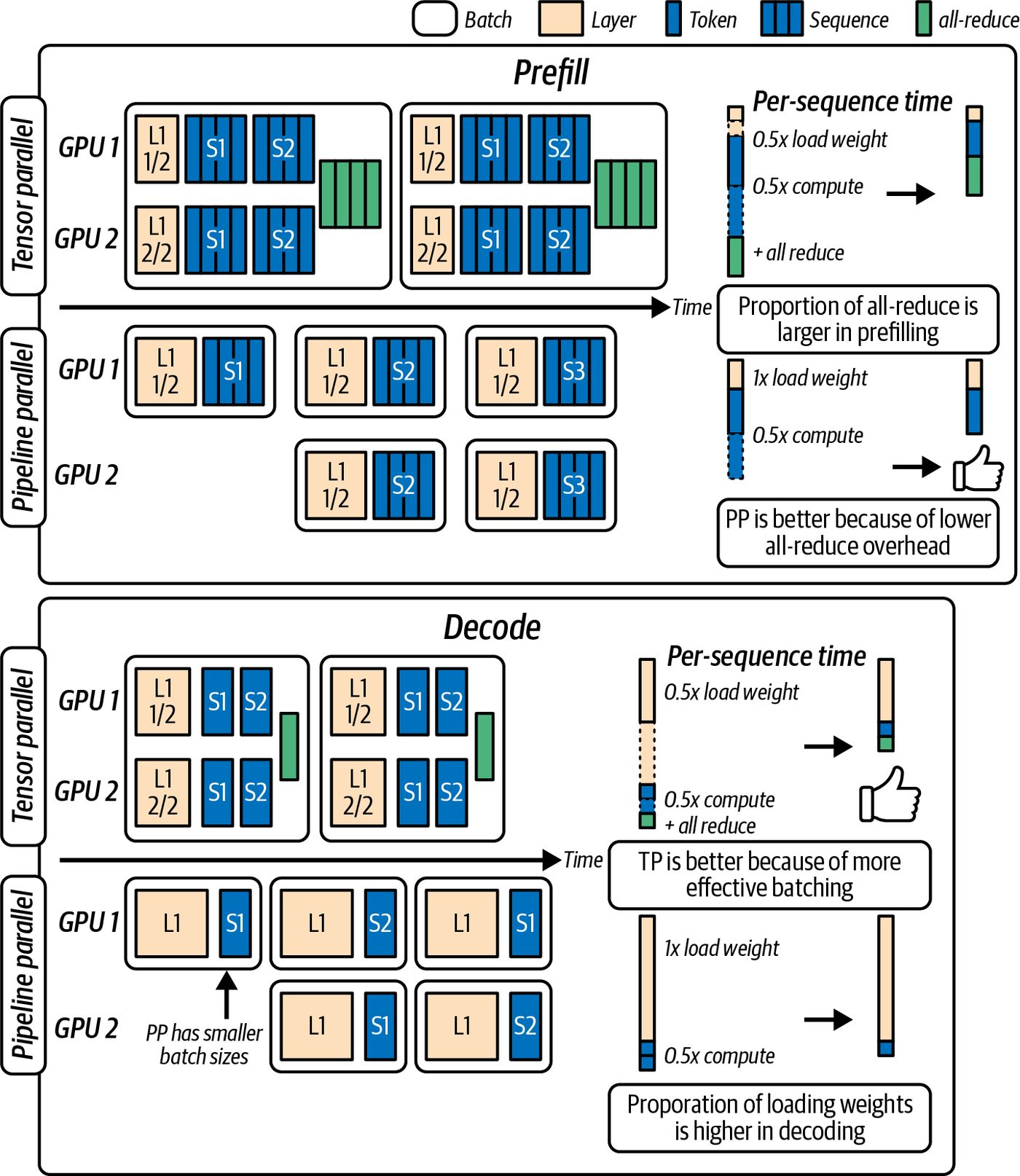
Phase-specific model parallelism Another form of heterogeneity and per-phase specialization is choosing different model parallelism (e.g., tensor parallel, pipeline parallel, etc.) across GPUs for each phase. This is relevant for very large models sharded across GPUs due to memory constraints. In a traditional setup, you might run the model with a fixed parallelism strategy and split the model across multiple GPUs using tensor parallelism or pipeline parallelism for both the prefill and decode phases. But the optimal parallelism strategy for prefill may not be the same for decode. For instance, the prefill phase is a big forward pass through N prompt tokens, and it benefits from a high degree of parallelization. You can use tensor parallelism (TP) across many GPUs to perform the computations faster and reduce TTFT. The overhead of synchronizing the GPUs is amortized over the large number of tokens that can be processed at once. This reduces the wall-clock time of this stage, which is critical for TTFT. You might even use pipeline parallelism (PP) to further speed up prefill and increase throughput. This would split the model layers across GPUs and stream the prompt through multiple pipeline stages. The decode phase, on the other hand, is sequential and latency-sensitive per step. Using too many GPUs for one decode can actually hurt time-per-output-token (TPOT) latency, also called inter-token latency (ITL). This is because each token step would require additional multi-GPU communication overhead. As such, the poten‐ tial for speedup is limited since there’s only one token’s worth of compute to split at a time (or a few tokens, if using speculative decoding). Disaggregation makes it possible to mix these approaches and use TP for one phase and PP for another—or use different degrees of each technique. For instance, you can run prefill with TP=8 to span 8 GPUs and minimize prompt latency. You can then run decode with TP=1, or a single GPU, to maximize per-token throughput and minimize
822 | Chapter 18: Advanced Prefill-Decode and KV Cache Tuning
step latency. In this way, each phase’s throughput and latency can be tuned separately, as shown in Figure 18-7.
Figure 18-7. Using different parallelism strategies for prefill and decode (source: https:// oreil.ly/1-Ti0)
Here, tensor parallelism’s additional all-reduce communication overhead is more prominent during the prefill stage since a large number of tokens are being processed in parallel. As such, we choose pipeline parallelism because it’s more efficient for our prefill workload.
Heterogeneous Hardware and Parallelism Strategies for Prefill and Decode | 823
                    Both tensor parallelism and pipeline parallelism can be effective for
                    prefill. The upcoming example uses pipeline parallelism for prefill.
                    However, a large tensor parallel degree can reduce TTFT on certain
                    clusters. The best choice depends on network bandwidth, collective
                    latency, and model shape.
For the decode phase, however, pipeline parallelism can lead to more, albeit smaller, forward passes as the tokens are passed between GPUs. This requires a lot of data movement in and out of the GPUs for just a single token generation. As such, we choose tensor parallelism because it’s better suited for our decoding workload. This introduces a complication, however. Since our model’s parallelization scheme differs between the prefill and decode, the format of the KV cache must differ as well. For instance, if the prefill phase uses TP = 1 (since it’s using PP) with four GPUs, each of the four GPUs has a full-size KV tensor. And let’s say the decode phase uses TP = 4. In this case, each GPU expects only 1/4 of the KV tensors since the data should be split up along the model’s hidden size. To handle this, systems like NVIDIA Dynamo can perform KV transposes, or conver‐ sions, during the transfer. Essentially, it converts and rearranges the KV cache from [TP_p parts] into the format needed by [TP_d parts], where TP_p is prefill’s paral‐ lel degree and TP_d is decode’s parallel degree. Dynamo includes a high-performance kernel to do this transpose on the fly after reading from NIXL—and before writing into the decode worker’s memory. This way, the receiving decode gets the KV cache data in the layout that it expects. The overhead of this transpose can be small compared to the network transfer, however—especially given NVLink throughput, which can handle these data reor‐ ganizations quickly. In this case, it’s easily justified by the compute savings of using different parallelism strategies optimized for each phase. Let’s explore an example of phase-specific parallelism. Consider a large model where we can apply various parallelism schemes: tensor (TP), pipeline (PP), data (DP), sequence (SP, splitting sequences across GPUs), etc. We might choose separate paral‐ lelism configurations. Table 18-1 shows an example parallelism configuration for the prefill phase.
824 | Chapter 18: Advanced Prefill-Decode and KV Cache Tuning
Table 18-1. Prefill parallelism example Parallelism Symbol Value Description strategy Tensor parallelism TP_p 2 Split the model’s weight tensors across 2 GPUs to halve prefill latency with manageable communication overhead. Pipeline PP_p 2 Divide the model layers into two pipeline stages, streaming microbatches through parallelism each stage for deep models. Sequence SP_p 1 Do not split the input sequence across GPUs (no sequence sharding) unless parallelism processing extremely large contexts. Context parallelism CP 1 Keep the entire context on a single GPU (no context-level partitioning) when it fits in memory after optimizations. Data parallelism DP_p 1 (or 2) Use one model replica per GPU (or two for doubled throughput on batched prompts by weight replication).
These numbers minimize inter-GPU overhead while still using multiple GPUs to speed up big prompts. Next, let’s look at an example parallelism strategy for decode, as shown in Table 18-2.
Table 18-2. Decode parallelism strategy example Parallelism Symbol Value Description strategy Tensor TP_d 1 (default) Default to TP_d = 1 for simplicity and minimal sync overhead. parallelism ... TP_d = N number of GPUs can improve efficiency for tiny GEMMs on small N (number of batches or when a single GPU can’t hold the model. GPUs) Pipeline PP_d 1 Pipeline parallelism adds bubbles for single-token decoding, so PP_d = 1 parallelism avoids idle stages. Sequence SP_d 1 Splitting the output sequence across GPUs is uncommon. parallelism SP_d = 1 keeps each decode stream local unless handling extremely long outputs. Data parallelism DP_d 1 One model replica per GPU per decode stream. Use separate replicas to handle parallel requests rather than replicating for a single stream.
                      If the model cannot fit on a single Blackwell B200, for instance,
                      prefer TP_d = 2 or 4 for decode instead of using PP. This will help
                      avoid pipeline bubbles.
Ideally, each decode stream runs on a single GPU and avoids cross-GPU overhead. This is possible only if the model fits into GPU memory. In this case, TP_d = 1, which means it’s not using any tensor parallelism during decode. If the model can’t fit into
Heterogeneous Hardware and Parallelism Strategies for Prefill and Decode | 825
memory, you can increase the degree of tensor parallelism (e.g., TP_d = N, where N is the number of GPUs). Increasing tensor parallelism is also useful if the system is issuing tiny GEMMs to process small batches. This is because distributing small matrix multiplications across devices can hide communication latency behind computation and potentially pro‐ duce higher overall throughput. These are illustrative values, but the main point is that disaggregation allows you to configure resources separately on the prompt side to reach a TTFT target. At the same time, you can independently adjust resources on the decode side to hit through‐ put and latency targets for streaming tokens back to the end user. This way, the two parallelism strategies do not interfere with each other. In a unified system, if you tried to do this, you’d have to pick one compromise strategy that works suboptimally for both phases.
Different precision for prefill and decode Some inference engines let you use different precision between prefill and decode. For example, you could perform prefill in a lower precision, such as FP8, INT8, or FP4, to speed it up. At the same time, you could decode in a higher precision if needed for better generation accuracy. Generally, you have both run in the same precision so that the KV cache computed in the prefill phase is usable in the decode phase. However, you can apply a conversion similar to the parallelism conversion described in the previous section. You would choose to quantize the KV and compress from FP16 to INT8/FP8/FP4 before send‐ ing. You would then convert it back on the receiving end, if needed. For instance, you can choose to send the lower precision over the network to speed up the transfer. Or you could choose to perform the conversion on the sender or receiver based on available FLOPS, etc. These are advanced ideas. But they highlight that nearly every aspect—hardware type, number of GPUs, and precision—can be independently tuned for each phase in a dis‐ aggregated setup.
Hybrid Prefill with GPU-CPU Collaboration So far, we have assumed that both the prefill and decode phases run on GPUs—and possibly different types of GPUs. However, at extreme scales—or with extremely large models and prompts—it’s worth evaluating if CPUs can offload pressure from GPUs. Modern CPUs are far slower than GPUs for neural network computations, but they come with other advantages like ample RAM, no contention for GPU memory bandwidth, and flexibility to handle tasks that GPUs might not handle as well, like
826 | Chapter 18: Advanced Prefill-Decode and KV Cache Tuning
extremely long sequences and nontransformer operations like tokenization, padding, etc. With a hybrid prefill strategy, part of the prefill computation is done on CPUs. One scenario is CPU offloading for superlong prompts. Consider a prompt with tens of thousands of tokens from a large document attachment. Even a powerful GPU might struggle to process such a large prompt due to memory constraints. In the case of extremely long prompts, the system could choose to perform the initial layers of the model on a CPU worker with lots of RAM to hold the long sequence. It would then stream intermediate results to a GPU later—or even perform the entire prefill on the CPU if latency isn’t an issue. The decode GPU would then receive the huge KV cache from the CPU worker.
               While not common in interactive inference, some batch or offline
               pipelines, like long-running “Deep Research” jobs, can use CPU
               preprocessing for very long texts.
A practical use of CPU offloading is processing background or low-priority prefill tasks. For instance, an LLM service might allow very large prompt submissions for offline processing of noninteractive requests. These could be assigned to CPU-only workers that eventually feed into a decode GPU for fast token generation. The latency would be high since CPUs are slower, but since it’s an offline job, this might be acceptable. And this configuration frees up GPU resources for more interactive workloads. Hybrid prefill is more common on CPU-GPU superchips like Grace Blackwell, in which the chip-to-chip interconnect is super fast. And it leverages the fact that CPU memory is massive compared to GPU memory. Imagine storing a gigantic KV cache in CPU memory with fast access from the GPU. A hybrid prefill would use the CPU’s memory to buffer or preprocess input tokens while the GPU focuses on the heavy transformer layers. A Grace Blackwell Superchip could handle a massive context by letting the CPU manage memory and initial layers and the GPU handle dense attention on chunks of the sequence. The Grace CPU could also be used to spill KV cache data that doesn’t fit in HBM into CPU DDR memory. This effectively extends the context length that the GPU can support. You can slice the transformer across devices by running the first N layers on the GPU in which the bulk of the tokens are handled and the sequence is essentially com‐ pressed. You would then offload the next M layers to the CPU, which has lots of
Hybrid Prefill with GPU-CPU Collaboration | 827
memory, before finally bringing the remaining layers back onto the GPU to generate the final outputs. This layer-partitioning technique adds significant data movement and orchestration complexity—and should be justified only in rare cases, such as ultralong contexts or severe GPU memory limits. Regardless, it shows how you can push hardware bound‐ aries in extreme inference scenarios. In our disaggregated architecture, involving CPUs would mean introducing a third kind of worker: the CPU prefill worker. The scheduling logic could then choose among three options: GPU prefill worker, CPU prefill worker, or local decode GPU prefill. The decision would depend on factors like prompt length or priority. For instance, the policy might be: if prompt_length > 5,000, route to a CPU prefill worker, knowing it will be slow but at least it won’t tie up GPUs and can use large memory. The decode stage would then wait longer for KV. Or possibly, in an extreme case, the decode could also be done on the CPU if truly offline. Generally, CPU offload would increase TTFT, so it’s not used for normal latencysensitive requests. It’s more of an extensibility and safety-net feature. If utilized, the system should monitor how often this path is taken, as frequent CPU offloads might indicate the need for more GPU capacity or model optimization instead. CPU offload also allows the system to handle edge cases like super long inputs or bursts when GPUs are all busy. It does this by falling back to the slower CPU rather than failing entirely. However, remember that it’s best to fail fast if the processing is too slow and exceeds SLO requirements. From a cost perspective, using CPUs for some work can be more economical since CPU cores are cheaper than GPU hours. Some cloud providers might run a mix of GPU and CPU instances for LLM serving. The CPUs perform input preprocessing— or even small model inferences—before engaging the GPUs. In short, while core disaggregation logic focuses on distributing work across GPUs, a robust ultrascale inference system can leverage CPUs in creative ways for certain parts of the workload. As hardware evolves and moves toward tightly coupled CPUGPU superchip designs like Grace Blackwell, the line between using a GPU and CPU will blur. Efficient scheduling should consider all available compute resources. The guiding principle remains the same, however. Use GPUs for what they do best, including mas‐ sive parallel compute on moderate sequence lengths. And use CPUs when GPUs might be inefficient, such as for extremely long sequences, memory-heavy tasks, or low-priority tasks.
828 | Chapter 18: Advanced Prefill-Decode and KV Cache Tuning
SLO-Aware Request Management and Fault Tolerance To hit SLO targets at ultrascale, it’s not enough to scale and schedule efficiently. Sometimes you need to also reject or defer work that would violate SLOs under the current load. We touched on this with Mooncake’s early rejection.
Early Rejection (Admission Control) Early rejection, or admission control, was introduced in Chapter 17. In short, it means that if the system predicts that it cannot serve a request within the latency tar‐ get, it will fail fast by returning an error or responding with “please try later.” This prediction can be based on current queue lengths, recent throughput, or even a light‐ weight ML model that forecasts response time. Early rejection is in contrast to queuing the request and then missing its SLO dead‐ line. This preserves goodput by making sure requests served by the inference system will meet their guarantees. In Mooncake, the early rejection strategy evaluates incoming requests against the estimated load on both the prefill and decode clusters. For instance, consider a decode cluster that is currently handling a large number of long sequences. When a new request arrives, and based on its expected output length, the system determines if decode utilization would surpass a safe threshold. Here, the system will immediately reject or defer that request and free up resources on the GPU node, as shown in Figure 18-8. By doing so, you prevent a situation where the request sits in the queue and then takes so long that it surpasses its latency SLO and slows down all other requests by consuming scarce compute or memory bandwidth resources. This reinforces the fact that it’s better to return a quick “too busy” response than to silently accept and then fail the latency guarantee. This is analogous to how web servers shed load under extreme overload to keep serv‐ ing the remaining requests with acceptable latency—the dreaded HTTP 503 error. This is better than timing out all requests.
SLO-Aware Request Management and Fault Tolerance | 829
Figure 18-8. Instance load when applying early rejection (source: https://oreil.ly/2xtK-)
830 | Chapter 18: Advanced Prefill-Decode and KV Cache Tuning
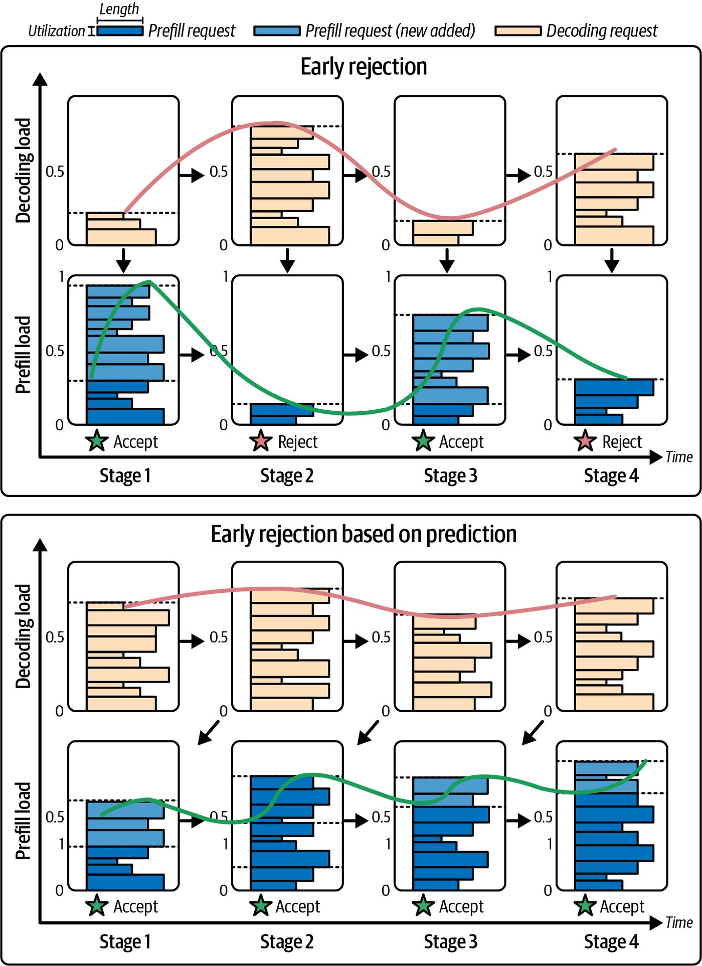
In LLM serving, because request sizes and durations vary widely, having a clear admission control step helps maintain performance for accepted requests. A wellbehaved admission control keeps the system in a regime where it can meet both TTFT and TPOT targets for the load that it has accepted. It effectively sets a limit on concurrent work. If doing more would break the SLO, it won’t attempt it. This must be combined with scaling policies. For instance, you can scale up rather than reject. However, since scale-up is typically not instantaneous—or you’re at max capacity—rejection is the safest and most performant option in the long run.
Quality of Service Another aspect of SLO-aware management is quality of service (QoS) differentiation. Some requests might include priority levels. For instance, paying customers have higher priority than free-tier customers. Or interactive queries have higher priority than offline batch requests. A scheduler might prioritize certain requests to always meet SLO—even if others have to wait or be dropped. Disaggregation can aid this by dedicating some portion of prefill and decode workers to high-priority tasks. For instance, you can choose to reserve 10% of cluster capacity exclusively for premium-tier requests and 30% for standard tier. This tiered approach will guarantee headroom for the paying tiers (premium and standard). It makes sure these requests aren’t delayed by lower-priority (free-tier) requests. Here is an example QoS configuration for NVIDIA Dynamo that demon‐ strates this type of tiered scheduling: # configs/qos.yaml
    scheduler:
      # Define QoS classes and their reserved capacity
      qos_classes:
        - name: premium
          reserved_fraction: 0.10   # reserve 10% of prefill/decode workers
          priority: 100
        - name: standard
          reserved_fraction: 0.30   # reserve 30% for standard tier
          priority: 50
        - name: free
          reserved_fraction: 0.60   # share remaining capacity (free tier)
          priority: 10
    # Map incoming requests to QoS classes by label
    request_router:
      routes:
        - match:
            header: "x-customer-tier: premium"
SLO-Aware Request Management and Fault Tolerance | 831
            qos: premium
          - match:
              header: "x-customer-tier: standard"
            qos: standard
          - match:
              header: "x-customer-tier: free"
            qos: free
          - match:
              # default fallback
            qos: free
This tiered approach allows higher-priority requests to be admitted and served with
low latency using reserved capacity. Lower-priority requests will be queued—or
potentially rejected—if the system is busy processing higher-priority requests.
Latency monitoring and feedback loops are useful for this type of system to continu‐
ously monitor TTFT and TPOT p99 and p99.9. If the system sees these metrics
approaching SLO limits, it can trigger actions such as scaling or rejecting new load,
degrading the requests by limiting the maximum output length, or temporarily
reducing the load.
In a disaggregated system, you can observe the prefill queue and decode the queue
separately. This helps pinpoint which side is the bottleneck. With this information,
the system can adjust accordingly by stopping to accept new prompts if prefill is
backed up or limiting long-output reasoning requests if decode is saturated.
                    You might have experienced “random” errors when using
                    ChatGPT. This can be for a number of reasons, but one of those
                    reasons could be these “circuit breakers” kicking in and shedding
                    load for certain types of requests when the system is under heavy
                    load.
Fault Tolerance Fault tolerance is another aspect of running a robust inference system. In a disaggre‐ gated system, if a decode node fails mid-generation, the KV cache pooling we dis‐ cussed earlier can enable recovery on another node since the KV was saved in the pool. This way, another decode worker can pick up generating the remaining tokens—perhaps with a slight delay. If the KV was not saved, the system will have to recalculate the prefill on another node and then continue with the decode. This is why systems like vLLM periodically checkpoint or copy the KV cache to the pool—even if disaggregation isn’t strictly needed. This is done to protect against failures.
832 | Chapter 18: Advanced Prefill-Decode and KV Cache Tuning
In addition to framework-level KV snapshots, a Linux process hosting a GPU worker can be suspended and snapshotted with cuda-checkpoint plus Checkpoint/Restore in Userspace (CRIU) as discussed in Chapter 5. This way, the checkpoint can be restored onto another node of the same GPU chip type to minimize work lost on preemption or failure.
                It’s possible reduce cold-start latency for inference engines by using
                cuda-checkpoint to restore prewarmed GPU memory rather than
                recompiling graphs and reloading weights on every start.
Checkpointing can hurt latency, but at least the request can complete. Prefill node failure is less impactful after it finishes computing and sending the KV data to either a decode worker or the KV cache pool since the KV data is off the failed node. But if the prefill worker fails during a prompt, the prompt task needs to be retried on another prefill node. The architecture should handle these types of failures gracefully so that one node’s failure doesn’t drop the entire request or cause large cascaded delays. In short, SLO-aware request management makes sure that even under extreme condi‐ tions, the system maintains performance guarantees for the load that it chooses to serve. It does this by intelligently deciding which requests to serve, which to shed, and which to delay. Early rejection is a concrete example that uses load prediction at admission time to prevent overload and maintain high throughput within the SLO constraints. SLO-aware request management and fault tolerance—combined with all the other strategies we’ve discussed so far (e.g., scaling, scheduling, and caching)—help main‐ tain strict SLO goals in production. Disaggregation makes this possible because it provides clear control points. You can observe prefill and decode metrics separately and apply admission controls specifi‐ cally where they’re needed. For instance, stop taking new prompts if the prefill cluster is backed up, or stop allowing long outputs if the decode cluster is at capacity. The result is a more predictable, stable, and adaptable inference service in which per‐ formance doesn’t degrade sharply when load exceeds capacity. Instead, it gracefully rejects excess load and rapidly rebalances to handle the changing conditions.
SLO-Aware Request Management and Fault Tolerance | 833
Dynamic Scheduling and Load Balancing Upfront, you can determine how many resources to dedicate to prefill versus decode. But then you want to dynamically adjust those resource splits as the workload changes. With a purely static configuration, if the workload mix changes and you require a more prompt-heavy or generation-heavy split, the fixed ratio will become subopti‐ mal. The optimal balance of prefill and decode capacity will shift over time. At one moment, many new requests arrive, and you want a heavy prefill split. Later on, you may have many long, ongoing reasoning generations, and you want a heavy decode split. Adaptive scheduling and load-balancing mechanisms aim to continuously tune the system so that neither phase becomes a bottleneck. This keeps goodput high under changing conditions. Modern inference engines like vLLM, SGLang, and NVIDIA Dynamo incorporate load monitoring and dynamic worker assignment into their platforms. In addition, many cloud inference platforms have custom autoscalers and routers that use similar principles.
Adaptive Resource Scheduling and Hotspot Prevention One issue with disaggregated setups is load imbalance between the prefill and decode clusters. If the ratio of prefill to decode workers is misconfigured for the current load mix, one side might saturate while the other side remains underutilized. For instance, if there are not enough decode workers relative to prefill, then decode tasks will queue up. This increases TPOT even though prompts are being processed quickly. Conversely, if decode is overprovisioned but prefill is underprovisioned, new requests may wait to start. This leads to high TTFT while many decode GPUs sit idle. The ideal scenario is when both sides are working near capacity but are not over‐ whelmed. This way the system keeps both prefill and decode busy but neither has a growing queue. Static prefill-decode worker allocations are not sufficient in real-world conditions because workloads can vary greatly throughout the day. The mix of input lengths and output lengths can vary significantly from hour to hour in a long-running, large-scale inference system.
834 | Chapter 18: Advanced Prefill-Decode and KV Cache Tuning
For instance, one hour might have a lot of long questions that produce short answers (e.g., summarization). These require more prefill resources and fewer decode resources. The next hour, you might get short questions that produce long answers (e.g., reasoning, web search). These require less prefill but much more decode. In other words, a static prefill-to-decode ratio that worked for one scenario may not be optimal for another. Thus, the optimal X_p versus Y_d configuration is workloaddependent and will shift over time. To address this, advanced inference systems can use adaptive scheduling algorithms that can redistribute load or even repurpose instances on the fly. Let’s discuss a few of these approaches next.
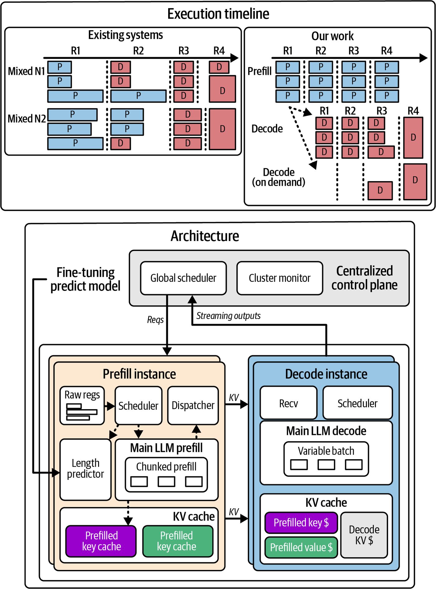
TetriInfer’s two-level scheduler The research prototype scheduler TetriInfer operates at two granularities. First, at the individual request level, it assigns incoming requests to specific prefill and decode instances based on current load. This is the normal routing that we expect. Second, it monitors resource utilization cluster-wide and predicts where bottlenecks might form. This proactively shifts work to prevent hotspots. For instance, the scheduler might see that one decode node is getting a bunch of very long sequences queued up. Before it becomes a problem, the scheduler routes some of those sequences to a different decode node that’s more available—even if it wouldn’t normally route to this decode node. This way, the load is balanced out. Figure 18-9 shows a comparison between existing systems and the TetriInfer work in terms of execution timeline and architecture. Here, you see that by predicting resource usage through queue lengths, GPU utiliza‐ tion trends, etc., TetriInfer’s two-level scheduler smooths out the load across the clus‐ ter and prevents any single node from being overloaded.
                 The name TetriInfer hints at “packing” requests like Tetris pieces to
                 fill GPU time without interference.
Dynamic Scheduling and Load Balancing | 835
Figure 18-9. Comparison between existing systems and TetriInfer’s architecture (source: https://oreil.ly/_3KGj)
836 | Chapter 18: Advanced Prefill-Decode and KV Cache Tuning
Arrow’s adaptive instance scaling Another technique for dynamic resource scheduling is Arrow (not to be confused with the popular Arrow data format). This is an adaptive instance scaling technique that leverages the fact that disaggregated systems often have a lagging response to workload changes. For instance, if the distribution of input versus output changes, the static number of prefill versus decode workers doesn’t immediately adjust. This causes a temporary loss of goodput since one side becomes a bottleneck. Arrow continuously analyzes the workload by measuring input token rate versus out‐ put token rate—and the backlog in each worker pool in the cluster. It then dynami‐ cally adjusts the allocation of workers, as shown in Figure 18-10.
Figure 18-10. Arrow architecture
In a cloud environment, this could mean spinning up additional decode instances when output load increases. You can also scale down decode in favor of more prefill instances if an input-heavy workload is detected.
Dynamic Scheduling and Load Balancing | 837
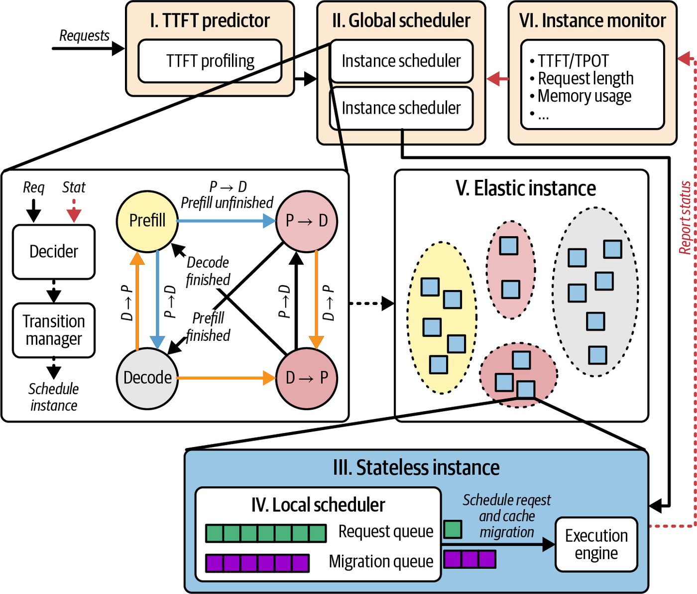
Arrow’s design includes both request scheduling to decide which node handles which requests (similar to other scheduling techniques) and instance scheduling to decide when to launch or shut down instances of either prefill or decode. Arrow treats the number of prefill and decode workers as a tunable parameter that can be adjusted and scaled in near-real-time. Arrow’s design brings an autoscaler logic inside the LLM inference scheduler. For instance, if a high volume of input-heavy but output-light requests come into the system, prefill nodes could become the bottleneck. In this case, Arrow would detect growing prefill queue times or rising TTFT percentiles and decide to convert some decode workers into prefill workers—or launch extra prefill instances to handle the surge. Conversely, if a wave of output-heavy requests with very long answers (e.g., reasoning chains) comes in, the decode cluster might start lagging, as indicated by TPOT rising and a long decode queue forming. In this case, Arrow could allocate more GPU workers to the decoding phase—perhaps by temporarily idling some prefill nodes if prompt arrivals have slowed. Otherwise, it could just add new decode nodes. In a static, on-premises cluster with a fixed number of GPUs, dynamic scaling will involve task reallocation by instructing a few GPUs that were assigned to prefill to switch roles and join the decode pool for a bit of time. This is feasible if each compute node is configured to run as both a prefill worker and a decode worker. There may be overhead to switching roles since the model may need to load different model partitions for different parallelism strategies or quantization choices, etc. Some designs keep all model weights loaded on every GPU and just feed them different tasks depending on the need. This effectively treats the cluster as a flexible pool where, at any given moment, some fraction of workers are doing prefill and others are doing decode. This starts to resemble a unified cluster with time-sharing but at a coarse granularity in which one node dedicates some time to performing prefill tasks, then switches to performing decode tasks. In cloud deployments, dynamic scaling can also mean interfacing with an autoscaler like the Kubernetes Horizontal Pod and Cluster Autoscalers to add or remove pods and nodes for each role. For instance, Arrow could trigger new prefill pods to start if the load is consistently high there. This leads to a fully elastic, disaggregated prefill and decode inference cluster that grows or shrinks each side as needed. In practice, scaling up new GPU pods can take tens of seconds or more. As such, the system may need to shed load while waiting for capacity. This is how Mooncake han‐ dles this situation, as we discuss next.
838 | Chapter 18: Advanced Prefill-Decode and KV Cache Tuning
Mooncake adaptive strategies Apart from Arrow, the Mooncake system also highlights adaptive strategies. Moon‐ cake introduced a prediction-based admission control called early rejection, which is somewhat complementary—managing demand versus managing supply. Specifically, if the system predicts it doesn’t have enough capacity to handle a new request within SLO, it will reject that request rather than accept the request and potentially violate the SLO. This is a form of dynamic load shedding rather than scal‐ ing, but it aims to prevent overload. We already covered Mooncake’s early rejection approach in the previous section. The point here is that adaptation can happen on the supply side by adding more resources or reallocating them—as well as on the demand side by throttling or rejecting some requests. The key benefit of dynamic scaling is maintaining high goodput across workload var‐ iations. By automatically tuning the prefill-to-decode ratio, the system avoids exten‐ ded periods of mismatch in which GPUs on one side are idle while the other side is overloaded. Ideally, both types of nodes are utilized evenly. This improves latency by alleviating bottlenecks as soon as they form—and also raises efficiency since you’re not paying for a bunch of idle GPUs of one type while the other type is overloaded. Instead, resources are reallocated or tasks shifted to keep things balanced. In terms of outcomes, an adaptive system might be able to claim something like, “After applying adaptive scaling, the system maintained > 90% SLO compliance across traffic patterns that a static system could not, and it handled X% more requests during a spike by quickly shifting resources.” Specifically, Arrow’s results mention an up to 5.6× higher request serving rate versus a nonadaptive system in a scenario with an extremely shifting workload. Typical improvements were lower but still significant. The exact improvement depends on how dramatic the workload changes are. All of this shows that disaggregation removes the phase interference issue. And dynamic disaggregation removes the next constraint of phase imbalance caused by a fixed allocation. To implement such adaptivity, the scheduler needs to monitor met‐ rics continuously, including the prefill queue length, decode queue length, and the TTFT/TPOT percentiles. These metrics are often fed into control dashboards using Prometheus and custom controllers in a K8s deployment. Algorithms can then auto‐ mate the decision making. Sophisticated inference systems use predictive models like ARIMA and other fore‐ casting techniques to foresee surges and predict traffic shifts using time-of-day pat‐ terns. If a spike of long outputs is predicted at 9 p.m. due to historically known usage
Dynamic Scheduling and Load Balancing | 839
patterns, the scheduler could preemptively allocate more decode capacity just in time. The overall goal is to maintain a high fraction of requests served within SLO—and without manual intervention and reconfiguration.
Dynamic resource scaling
Building on the idea of predictive scheduling, dynamic resource scaling is specifically
about changing the distribution of resources between prefill and decode in response
to load. For example, Arrow’s adaptive instance scheduling adjusts the number of
prefill versus decode workers continuously. Here are some ways to balance the load in
an inference system:
Elastic instances
    In Kubernetes or similar, you can define an autoscale policy for each deployment.
    For example, you can specify that you want to maintain average prefill GPU uti‐
    lization at 70%. If GPU utilization goes higher, the system will add a pod or node
    to the prefill worker pool. If it goes lower and decode utilization remains high,
    the system can move one pod from prefill to decode. This could be rule-based or
    algorithmic, such as solving for the most optimal configuration at each interval
    to choose new X and Y counts.
Instance “flip” mechanism
     The TetriInfer paper describes an “instance flip” in which some nodes can flip
     roles if needed. This requires that the model be loaded, sharded, and quantized
     properly to handle both roles.
Statelessness for elasticity
     Arrow leverages stateless instances. As such, no long-lived session state is stored
     on the worker. This way, they can be reassigned freely. The KV cache of active
     requests complicates flipping a decode node to prefill if it’s mid-token-
     generation, so you often have to wait until the decode finishes its task before
     switching roles.
Stability and oscillation
    Rapidly switching roles can lead to oscillation and thrashing. As such, it’s com‐
    mon to enforce some minimum amount of time required for a role to avoid flip‐
    ping too frequently.
Apart from load balancing, another aspect to consider is multitenancy or mixed
workloads. If the cluster serves different models or tasks, you can even repurpose
GPUs between them based on demand—and beyond a single model’s scope.
Disaggregation’s modular configuration allows using idle decode GPUs to run
another smaller model’s inference tasks. This is an extension that is not yet main‐
stream as of this writing, but it’s conceptually possible as inference engines evolve and
become more flexible in their designs.
840 | Chapter 18: Advanced Prefill-Decode and KV Cache Tuning
The bottom line is that an ultrascale inference system requires a feedback loop to continually match resource allocation to the current workload. TetriInfer, Arrow, Mooncake, and others show significant improvements when using such a feedback loop and adapting to load changes. This highlights that while disaggregation removes interference, adaptive disaggregation removes imbalance. Both are needed for the best performance under dynamic conditions.
Key Takeaways
This chapter covered various techniques, such as unified megakernels, efficient mem‐
ory allocations, fast data transfers, prefill/decode disaggregation, KV cache pools,
dynamic scaling, and continuous SLO awareness. Here are some key takeaways:
Accelerate the decode phase
    The decode phase can be greatly accelerated using fused attention kernels includ‐
    ing FlashMLA, ThunderMLA, and FlexDecoding. These kernels can improve
    single-token throughput and GPU utilization.
Treat the KV cache as a first-class citizen
    Share the KV cache across GPUs using disaggregation. Reuse prefixes to avoid
    redundant computation. These are enabled by global cache pools and hashing.
Strive for near-zero overhead between prefill and decode workers
     Leverage high-speed GPU-to-GPU transfers with GPUDirect RDMA and NIXL.
     Overlap compute/transfer to achieve near-zero overhead between prefill and
     decode workers.
Embrace specialized hardware and parallelism for each phase
   Disaggregating prefill and decode allows specialized hardware and parallelism
   per phase. For example, use high-compute GPUs or multi-GPU nodes for prefill.
   And use memory-rich GPUs or single GPUs for decode. The goal is to reduce
   cost and increase throughput.
Use adaptive and dynamic algorithms to optimize the system
    Adaptive scheduling and SLO-aware control (e.g., early rejection and dynamic
    scaling) are necessary to maintain latency guarantees under varying load—and to
    fully utilize all GPUs without overload.
Conclusion Ultrascale LLM inference requires a holistic approach, including both high-level adaptive resource management and low-level kernel and memory optimizations. By combining the techniques presented in this chapter, a highly optimized inference deployment can achieve maximum throughput on modern hardware while meeting strict latency guarantees.
Conclusion | 841
As hardware continues to evolve and GPUs (e.g., increased memory and specialized inference cores) and software frameworks become more sophisticated (e.g., dynamic routing and flexible role assignments), these optimizations will compound and become even more powerful. This will allow inference engines to efficiently handle even larger models, longer contexts, and more users.