Ch 17 — Scaling Disaggregated Prefill and Decode for Inference
As mentioned in an earlier chapter, LLM inference can be divided into two distinct phases: the prefill phase and the decode phase. The prefill phase processes the input prompt to produce the model’s internal key-value (KV) cache for that prompt, while the decode phase generates output tokens one by one—or a few at a time, in the case of speculative decoding—using those cached values. These two phases have fundamentally different performance characteristics. The pre‐ fill phase is compute bound, involves heavy matrix multiplications over potentially thousands of tokens in parallel, and consumes a significant amount of FLOPS. In contrast, the decode phase is memory I/O bound, reads the large KV cache for each token generation, writes new values, and stresses memory bandwidth. In simpler terms, prefill is a high-throughput, parallel workload, whereas decode is a sequential, latency-sensitive workload. Early LLM serving systems treated the two phases as one monolithic pipeline on the same hardware. As such, they typically favored the prefill phase by prioritizing throughput using request batching. However, as interactive applications grew, latency metrics like time to first token (TTFT, or prefill latency for all tokens) and time per output token (TPOT, or decode latency per token) became as important as raw throughput. It’s difficult for a single GPU-based inference engine to optimize both TTFT and TPOT simultaneously when serving both phases together.
Batching many requests will improve throughput but will worsen TTFT since every request waits for the slowest prefill. It will also impact TPOT since the decode steps will get backlogged behind new-prompt prefills. Monolithic inference systems must choose between improving (reducing) time to first token at the cost of slower subsequent token generation—or improving (increas‐ ing) per-token throughput while subjecting new requests to high initial latency. In extreme cases, one long prompt can completely tie up the GPU, which would block all other prompt prefill work for other users. And then, once decoding begins, the one-token-at-a-time processing would leave the GPU’s cores idle between each token generation. To address these issues, researchers and engineers looked for ways to decouple the two phases. The key insight is that prefill and decode do not actually need to run on the same hardware—or even the same type of hardware. Disaggregating the prefill and decode phases means assigning them to different resources that are each specialized for the needs of that specific phase. This idea was pioneered by systems in a paper on DistServe, which demonstrated that by eliminat‐ ing interference between the phases, one can meet strict latency requirements for both TTFT and TPOT simultaneously. DistServe’s evaluation showed the potential for serving 7.4× more requests within strict latency service-level objectives (SLOs) compared to a state-of-the-art baseline without prefill/decode disaggregation. As such, industry frameworks began to experi‐ ment with separate prefill and decode servers. The open source vLLM library introduced disaggregated operation in conjunction with LMCache and other components. NVIDIA’s Dynamo implements disaggregated prefill and decode with dynamic routing and autoscaling and publicly documents operational details. Many providers and open frameworks implement or evaluate dis‐ aggregation. For instance, to meet strict latency SLOs, industry-scale serving systems from OpenAI, Meta, and xAI have reportedly adopted this disaggregated approach. As such, disaggregated prefill and decode is standard practice for LLM inference at scale. At ultrascale, large inference deployments can involve hundreds of thousands or even millions of GPUs serving billions of requests. In these environments, the cost and performance benefits of disaggregation are massive. By splitting the workload, you can optimize each phase in isolation and avoid one of them becoming the bottleneck for the other. The remainder of this chapter explores how to design and operate a disaggregated prefill/decode inference system at extreme scale.
760 | Chapter 17: Scaling Disaggregated Prefill and Decode for Inference
In this chapter, we will explore scheduling algorithms to route requests between pre‐ fill and decode workers, techniques to maintain quality of service (QoS) under heavy load, and mechanisms that make this separation efficient. We’ll explore everything from high-speed interconnects to specialized decoding kernels. We will also discuss heterogeneous hardware strategies that use different GPU types for each phase.
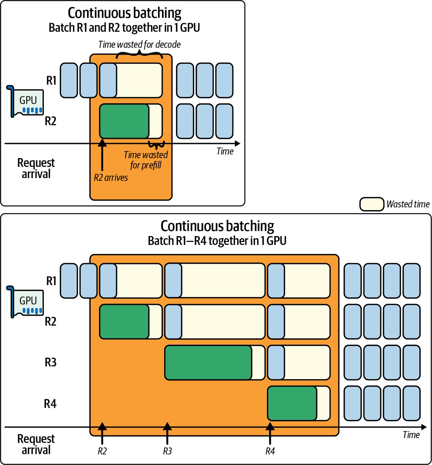
Why Prefill-Decode Disaggregation? Modern interactive LLM services often target TTFT latency < 200–300 ms for p99 (99% of requests). This is nearly impossible to guarantee without separating the pre‐ fill work since a one-size-fits-all approach to LLM serving leaves significant perfor‐ mance on the table. For context, the MLPerf v5.0’s (2025) inference benchmark for Llama2 70B (70 billion parameters) aimed for p99 (99th percentile) SLOs of ~450 ms TTFT and 40 ms TPOT latency. For Llama 3.1 405B (405 billion parameters), the benchmark aimed for ~6 seconds TTFT and 175 ms for TPOT. Specifically, these SLOs reflect p99 TTFT and p99 TPOT targets for Llama 2 Chat 70B and Llama 3.1 405B Instruct. Consider a scenario in which one user’s request has an extremely long prompt on the order of many thousands of tokens—and another user’s request has a very short prompt. Without disaggregated prefill and decode, if these requests arrive around the same time, the long prompt’s prefill computation will block the GPU for an extended period. Without disaggregation, the second request with the short prompt needs to wait an unnecessarily long time before even starting their decode. This is called interference since the prefill work for one request delays the decode work of another. Interference between prefill and decode is shown in Figure 17-1 in the context of continuous batching. Under a simple FIFO scheduling strategy, long prompts can amplify tail latency for everyone. In general, long or compute-heavy prefills at the front of the queue will block shorter, lighter requests behind them. This is called head-of-line blocking, and it leads to poor utilization, latency outliers, and unhappy end users. In a flexible disaggregated architecture, it’s possible to send a large prompt prefill to the dedicated pool of compute-optimized prefill workers, while a lightweight prompt prefill can be sent to the decode workers directly—bypassing the prefill workers. This type of flexibility allows shorter tokens to not suffer from head-of-line blocking. This maximizes overall throughput and minimizes latency tail effects.
Why Prefill-Decode Disaggregation? | 761
Figure 17-1. Interference caused by colocated prefill and decode running on the same GPU (source: https://oreil.ly/GRkHs)
Advantages of Disaggregation Disaggregation has two primary advantages: reduced interference and phase-specific optimizations. Let’s discuss each of these next.
Reduced interference With disaggregation, prefill tasks no longer contend with decode tasks on the same device. A busy decode worker, generating many tokens, won’t prevent another user’s prompt from being processed, and vice versa.
762 | Chapter 17: Scaling Disaggregated Prefill and Decode for Inference
Dedicated resources for each stage mean a long prompt’s computation won’t block another user’s token generation. In practice, this produces more predictable latency. Figure 17-2 shows the comparison between colocated and disaggregated prefill and decode. This experiment is described in more detail in the DistServe paper and subse‐ quent blog post by the authors.
Figure 17-2. Comparison between colocated and disaggregated prefill and decode (source: https://oreil.ly/GRkHs)
Here, the SLO is set to 0.4 seconds for P90 TTFT and 0.04 seconds for P90 TPOT (e.g., horizontal line in Figure 17-2). The colocated system can support only ~3 requests per second (RPS) of goodput within the given TTFT latency bounds. And it can sustain only 1.6 RPS within the given TPOT latency bounds. As such, the good‐ put of the colocated configuration is only 1.6 RPS since both the TTFT and TPOT latency SLOs need to be met. After disaggregating the two stages and assigning two prefill workers (two GPUs) and a single decode worker (one GPU), called a 2P1D configuration, both the prefill and decode workers achieve better overall RPS than the colocated configuration with a single GPU. Specifically, the prefill worker reaches ~5.6 RPS and the decode worker
Why Prefill-Decode Disaggregation? | 763
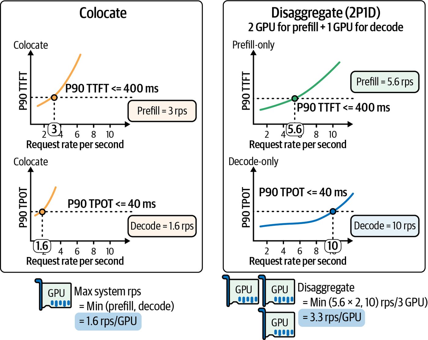
achieves ~10 RPS spread across the three GPUs. As such, the goodput for the 2P1D configuration is 3.3 RPS per GPU. The 3.3 RPS per GPU is calculated by taking the minimum of the RPS of the prefill workers (5.6 RPS × 2 = 11.2 RPS) and the decode worker (10 RPS). This is 10 RPS total across all three GPUs. As such, we have to divide the RPS by the number of GPUs, or 3 in this case. Under the configured SLOs, this system’s goodput result is 10 RPS ÷ 3 GPUs = 3.3 RPS per GPU.
                    In this comparison, the decode side improvements primarily
                    impact per-token latency. Meanwhile, prefill isolation primarily
                    improves time to first token. Both SLOs must be satisfied to count
                    as goodput.
This isolation can also improve tail latencies as well. Empirically, systems that disag‐ gregate show tighter latency distributions—and avoid the long tails seen in mono‐ lithic systems. By eliminating cross-phase interference, each phase meets its SLO more reliably—and with more predictable consistency. Now, you should also be asking, “Is the 3× cost worth the 2× improvement?” And you would be right to ask that. Additional tuning is required to make this solution more cost-effective, but it shows the right direction to tighten latency distributions and improve goodput. You need to decide based on your workload. Disaggregation is a popular option to meet goodput RPS needs.
Phase-specific optimizations Phase-specific optimizations let each phase use the hardware and parallelism that suits it best. The prefill phase, for instance, is compute bound. As such, you’d typically increase tensor parallelism to drive peak FLOPS on a high-FLOPS GPU. Additionally, modern GPUs provide lower precision modes (FP8 and FP4) that can increase throughput for the compute-heavy prefill phase.
                    You should prefer FP4 for weights and, where validated, activa‐
                    tions, as well. Many stacks use FP4 for weights and FP8 for activa‐
                    tions. These reduced precisions help to maximize throughput and
                    minimize HBM footprint—with minimal accuracy loss. These pre‐
                    cisions are supported by modern hardware and software stacks,
                    including the NVIDIA Tensor Cores and Transformer Engine.
In contrast, the decode phase is memory-bandwidth-bound and suffers from crossGPU synchronization overhead. So it’s most efficient with little or no tensor parallel‐ ism (often TP=1) as it relies more on fused kernels to increase arithmetic intensity—as well as high memory throughput GPUs.
764 | Chapter 17: Scaling Disaggregated Prefill and Decode for Inference
In a monolith you’d have to pick one type of GPU and one parallelism strategy for both phases, which is suboptimal for at least one of the phases. Disaggregation, on the other hand, lets you independently tune each phase for maximum efficiency. Splitting phases also opens the door to heterogeneous clusters in which different GPU types are assigned to prefill and decode roles for optimal cost-performance. For example, using compute-optimized GPUs for prompt prefill and memory-optimized GPUs for token generation can produce better throughput per dollar than a homoge‐ neous deployment.
               In practice, the latest GPUs typically have both higher FLOPS and
               more GPU memory. As such, it’s tempting—and more common—
               to just use the latest GPU generation for both prefill and decode.
               But just know that heterogeneity is a viable option to reduce cost.
We will explore the idea of heterogeneous clusters later in the chapter. We’ll show how using high-end GPUs for prompts and cheaper GPUs for generation can lead to significant cost savings at scale. In summary, disaggregation removes cross-interference and enables specialized treat‐ ment of each phase. The expected results include tighter latency distributions since no more long tails are caused by mismatched prompt sizes, improved throughput under latency constraints (goodput), and better overall resource utilization.
               You should use profiling tools (e.g., NVIDIA Nsight Systems) to
               identify bottlenecks in the prefill and decode phases. These can
               trace GPU kernels and RDMA transfers across the different worker
               nodes. This will help validate that decode kernels are fully overlap‐
               ping communication, etc.
Next, let’s discuss how to actually implement a disaggregated serving system, includ‐ ing the system architecture, communication, and scheduling policies that decide how to fully utilize the disaggregated cluster.
Disaggregated Prefill and Decode Cluster Pools In a disaggregated deployment, we maintain two (or more) pools of workers such that one set of GPUs is dedicated to prefill prompt processing and another set is dedi‐ cated to token generation. These workers can be on separate nodes or racks in a data center—or even in separate data centers if the interconnect is fast enough. (Note: keeping prefill and decode within the same data center is the practical design choice to achieve realistic SLOs.)
Why Prefill-Decode Disaggregation? | 765
The worker pools communicate over a network to hand off the model’s KV cache produced by the prefill to whichever GPU will perform the decode. A scheduler, or router, coordinates this communication. Consider a configuration in which the model weights are loaded on two groups of GPU servers. One group, the prefill workers, handles prompts and computes the KV cache. The other group, the decode workers, handles token generation using the KV caches generated from the prefill workers. The two worker groups typically communicate using a high-speed interconnect (e.g., NVLink/NVSwitch and InfiniBand) and zero-copy GPU-to-GPU transfers with RDMA. In practice, these transfers use GPUDirect RDMA or UCX and can be corre‐ lated in Nsight Systems alongside CUDA kernels, NVLink activity, storage metrics, and InfiniBand switch metrics for end-to-end validation.
                     For superchip-based NVL fabrics (e.g., Grace-Blackwell, Vera-
                     Rubin, etc.), use NVIDIA Multi-Node NVLink (MNNVL), keep
                     NVLink-first collectives enabled for TP decode, and enable SHARP
                     for AllGather and ReduceScatter collectives when available.
When the system receives a new request, it typically receives it on the decode worker. This is called a decode-centric design. This is preferred because the prefill workers are already compute bound with the KV computations. By having the decode workers handle the client I/O, routing, and session state man‐ agement, the inference system avoids overloading the prefill workers. Also, centraliz‐ ing request ingress on the decode nodes simplifies network management, autoscaling, and policy enforcement.
                     This is just one style of system architecture for prefill-decode in
                     which the decode worker is the centralized ingress for all requests.
                     This architecture is used in the NVIDIA Dynamo inference system.
                     Another common architecture is to use a dedicated, centralized
                     API router to route the request to either the prefill or decode
                     worker. However, this requires an extra moving part in the system
                     and additional coordination between the router and prefill/decode
                     workers, —as well as additional scaling and latency considerations.
After the decode worker receives the requests, it decides whether to do the prefill itself or “offload” it to the prefill worker pool. If it decides to offload to the prefill worker pool, the decode worker will later receive the KV results back and then continue with decoding and generating the next token.
766 | Chapter 17: Scaling Disaggregated Prefill and Decode for Inference
Next is a snippet from a simplified NVIDIA Dynamo cluster configuration that
defines two roles that use NVIDIA’s Inference Xfer Library (NIXL) for GPUDirect
RDMA-based KV cache transfers to let one GPU write into another GPU’s memory
directly over the network:
    roles:
      - name: prefill_worker     # Prefill worker role
        model_path: models/llm-70b
        instance_count: 4        # 4 prefill workers
        gpu_type: B200           # B200 Blackwell compute-bound prefill
      - name: decode_worker      # Decode worker role
        model_path: models/llm-70b
        instance_count: 8        # 8 decode workers
        gpu_type: B300           # B300 Blackwell Ultra high-memory decode
                NVIDIA’s Rubin CPX accelerator is another option for prefill
                workers. Rubin CPX (the CP stands for “context processing”) is
                specifically designed for compute-bound workloads such as prefill.
                The Rubin CPX marks NVIDIA’s departure from “general acceler‐
                ated computing” GPUs into specialized chips that are optimized for
                a specific stage (e.g., prefill) within a broader AI workload such as
                inference.
In this configuration, we have four prefill workers using B200 GPUs (adequate com‐ pute for compute-heavy prefills) and eight decode workers using B300 GPUs (high HBM capacity for heavy memory-bound decodes). Mixing B200s and B300s helps to match their FLOPS and HBM capacity characteristics while minimizing cost. Both roles will use NIXL and GPUDirect RDMA to transfer the KV cache blocks. NIXL abstracts transport for GPU-to-GPU data movement over NVLink and RDMA NICs. It also provides connectors for GPUDirect Storage so that KV cache pages can be read from (or written to) different storage tiers. Under the hood, when this system runs, each decode worker registers a region of its GPU memory so that prefill workers can write directly into it using RDMA. Typically, memory-registration metadata such as NIXL descriptors are exchanged at startup or on first contact. This way, for each remote prefill task, only a small identifier needs to be sent rather than a full memory address structure. For instance, Dynamo uses etcd for worker discovery and leases. Workers register the necessary memory handles with the router or control plane so that peers can obtain the descriptors when needed. The prefill workers will retrieve them on first use. This way, a prefill request can include just an ID for the target KV buffer, making control messages lightweight.
Why Prefill-Decode Disaggregation? | 767
Furthermore, NVIDIA Dynamo’s NIXL implementation provides a high throughput RDMA and storage abstraction for inference data movement and includes plugins for NVLink, UCX-based fabric, and GPUDirect Storage. As such, prefill workers can write KV blocks directly into decode GPU memory.
                     In mixed parallelism deployments where prefill and decode use dif‐
                     ferent TP layouts, you need to perform a layout transform on the
                     decode side immediately after the NIXL read. This way, the KV
                     pages match the decode kernel’s expected layout. This transform is
                     latency-insignificant compared to network transfer and avoids
                     re-prefill.
This architecture decouples scaling for each phase. If you find that prefill is the throughput bottleneck due to many concurrent long prompts, for instance, you can add more prefill workers to increase prompt processing capacity. If decode becomes the bottleneck due to many users generating long outputs, for instance, you would scale out decode workers. Because decode and prefill are separa‐ ted, scaling one doesn’t directly interfere with the other. Systems like NVIDIA Dynamo support dynamic, runtime-configurable disaggrega‐ tion such that you can add or remove prefill workers on the fly—without stopping the cluster. New prefill workers simply register and start pulling tasks from the queue. If a prefill worker leaves the cluster for whatever reason (crash, restart, autoscale event, network partition, etc.), the decode workers will temporarily do more local prefills to compensate. NVIDIA Dynamo’s distributed runtime uses etcd for worker discovery and leases. Its Planner component can scale workers by revoking leases or launching new workers which are auto-discovered. This dynamic flexibility is crucial at ultrascale when load will often fluctuate. When this happens, you’ll want to swap workers between roles as needed.
Prefill workers design Prefill workers, or prompt servers, are the compute nodes dedicated to executing the initial prompt prefill processing phase of requests. This section discusses how prefill nodes are architected to handle the heavy computation efficiently—and how they bal‐ ance latency versus throughput for KV cache population under load. Because the prefill workload is computationally intensive, prefill nodes should use GPUs with high FLOPS and be optimized for large matrix multiplications. Each pre‐ fill task feeds n input tokens through all model layers.
768 | Chapter 17: Scaling Disaggregated Prefill and Decode for Inference
The prefill workers will use thousands of GPU threads in parallel—and across many GPU nodes, if available. They use familiar parallelism techniques, including tensor parallelism and pipeline parallelism, to reduce TTFT.
Memory management. Memory-wise, prefill nodes need to load the full model weights and also allocate KV cache for the prompt. This KV cache is then transferred to the decode workers, as we’ll see in a bit. Prefill populates GPU memory with model parameters and the working activations of the model’s forward pass with the prompt inputs. Once the KV cache is created, it’s immediately sent to the decode workers. The KV cache doesn’t persist long in the prefill node’s memory. If a model is extremely large or a prompt is extremely long, prefill may require tensor or parallel splits across GPUs due to memory limitations. Prefill servers should be flexible with their parallelism strategies (data, tensor, pipeline, expert (MoE), and context) to meet latency targets. Some inference frameworks preallocate a big chunk of GPU memory for prefills to use as working space. This reduces overall memory fragmentation and buffer alloca‐ tion time.
Optimizing for latency versus throughput. When tuning a disaggregated prefill cluster,
you face a fundamental trade-off between minimizing the TTFT for each individual
prompt and maximizing overall requests per second (RPS), or reducing TPOT, under
heavy load.
Disaggregated systems handle this trade-off by supporting different scheduling poli‐
cies for a latency-first approach versus a throughput-first approach. Let’s describe
each of these approaches next:
Latency-first approach
    To reduce TTFT, prefill nodes should process prompts as soon as they arrive—
    and with little to no batching. In this mode, you avoid waiting for other requests
    to fill a batch. As such, every prompt starts execution immediately and finishes as
    fast as possible—assuming available GPUs in the cluster.
    The downside of this latency-first approach is lower GPU utilization since you
    are using small or no batches. As such, GPUs often sit idle, and your system will
    serve fewer concurrent requests for a given cluster size. In this case, you can
    either over-provision your prefill cluster capacity or use a tiny batch size of 1 to
    guarantee strict latency SLOs for your requests.
Throughput-first approach
    If peak throughput, or RPS, and minimal TPOT are your priorities, you should
    batch prompts into larger groups to fully load each GPU. By accumulating 8–32
Why Prefill-Decode Disaggregation? | 769
prompts into a single batch, you raise arithmetic intensity and keep the GPU compute units busy. This will increase the overall throughput. The downside to the throughput-first approach is that each request incurs a batching delay equal to the time it takes to collect the batch. The larger the batch size, the longer the delay. For extreme throughput inference system configurations, you can choose to assign multiple GPUs per request using either data parallelism or pipeline paral‐ lelism. With data parallelism, the entire model is replicated on each GPU. The batch is split into minibatches across the GPUs. Each GPU performs a forward pass on its subset of data through its complete copy of the model. The output is then aggregated from all the GPUs for the final output. Data parallelism aggregates memory bandwidth and compute power across all of the GPUs to increase per-batch performance. However, it reduces maximum parallelism to the total # of GPUs ÷ GPUs per request. This reduces your overall concurrent request capacity. This can leave resources idle if the system uses too many GPUs per single request. This will create an imbalance between throughput and concurrency. Pipeline parallelism divides the model’s layers into sequential stages on different GPUs, such as GPU 0 and GPU 1. As soon as GPU 0 finishes its stage for microbatch 0, it forwards activations to GPU 1 and begins stage 1 for microbatch 1. This assembly-line pattern keeps all GPUs busy on different chunks of work. Pipeline parallelism increases per-batch throughput, but it adds inter-GPU commu‐ nication overhead and pipeline “bubbles” if the microbatch size or stage splits are not carefully balanced. Ultimately, each additional GPU that you dedicate will increase throughput but decrease how many requests you can handle at once—given a fixed-size cluster. You can always scale out the GPU cluster, but assuming a fixed cluster size, you should choose your configuration based on whether latency SLOs or throughput SLOs are most important to your use case.
Latency-aware scheduling and batching. Disaggregated systems incorporate the latencyaware scheduling policies mentioned earlier to balance these factors. For instance, they might guarantee single-request execution—and not batch requests—unless load is high enough that combining a small number of requests won’t violate the TTFT target. Many cluster designs include an SLO constraint in the scheduler. For instance, if p90 TTFT must be ≤ X ms, the system will choose the largest batch size or parallelism strategy that still meets the SLO for a typical prompt size.
770 | Chapter 17: Scaling Disaggregated Prefill and Decode for Inference
Another strategy is adaptive batching windows. For instance, at low load, it can run requests immediately using a batch size of 1. And at higher loads, the system can allow microbatches of requests arriving within a small time window, such as 2–10 ms. This way, a slight delay can produce a big GPU utilization win—but only when it’s needed and tolerable. Many inference engines favor latency for their prefill workers. Systems often execute prompt tasks as soon as possible and even tolerate some GPU underutilization, because a fast first token significantly improves user experience. It’s common to provision more prefill capacity than needed for an average load. This way, the prefill cluster absorbs bursts of prompts without latency spikes. In the next chapter, we will discuss adaptive mechanisms to rebalance resources on the fly so that neither the prefill nor the decode workers become a bottleneck over time. Modern orchestrators like Kubernetes can automatically scale each tier. For example, if prefill GPU utilization stays high and decode is low, the orchestrator can trigger an autoscaling event to add prefill pods (or nodes)—and possibly even remove some decode pods/nodes.
               This kind of adaptive scaling is often implemented with metrics
               like prefill queue length to help drive the decisions.
Another option is to implement priority queues such that short prompts are sched‐ uled on a separate fast lane with less batching. Long, batchable prompts go to a throughput-optimized queue. NVIDIA Dynamo supports latency classes in schedul‐ ing. You can emulate this by tagging requests and having different batching windows per class. The key takeaway is that prefill workers prioritize quick turnaround. Disaggregation lets us do this without harming decode performance since decode is running on a dif‐ ferent set of workers. We might “waste” some prefill GPU cycles during low-traffic periods, but we maintain low TTFT during peak traffic periods. It’s a worthwhile trade-off for interactive services.
Decode workers design Decode workers, or generation servers, are dedicated to the autoregressive decode phase. Once a prompt’s KV cache is ready, it is sent to a decode worker, which uses the KV cache to produce the remaining output tokens as quickly as possible to main‐ tain a low TPOT latency.
Why Prefill-Decode Disaggregation? | 771
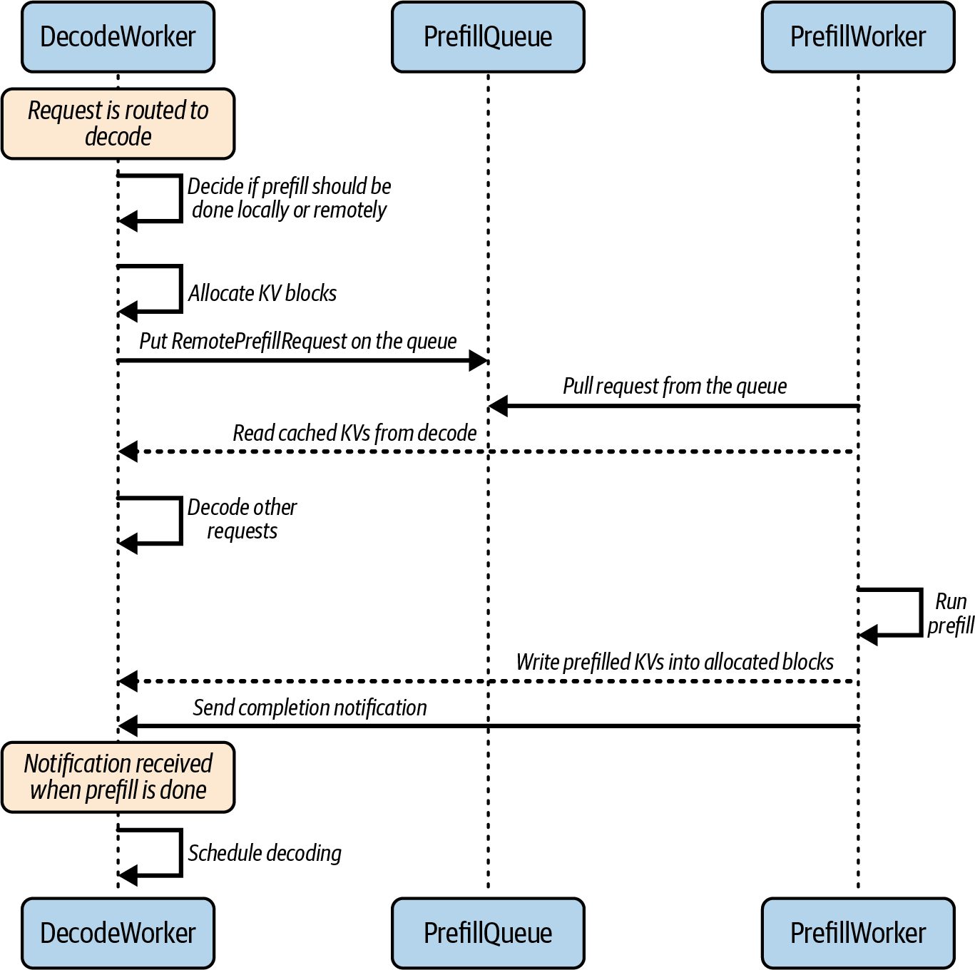
If a request is initially routed to the decode worker, as in Figure 17-3, it must first decide if the prefill should be done locally or remotely using a disaggregated router. If it decides to prefill remotely, it will push the prefill request into a prefill queue to be picked up by the prefill worker. The prefill worker continuously pulls from the prefill queue, reads any KV blocks cached in the prefix cache, and computes the prefill operations. It then writes the KV blocks back to the decode worker, which completes the decoding.
Figure 17-3. Prefill worker design: read prefix cache → compute prefill → write KV cache for decode
The decode worker design is focused on handling many concurrent sequence genera‐ tions efficiently—as well as managing the memory footprint of the KV cache. In this section, we describe how decode servers achieve high throughput using techniques like continuous batching and clever memory management tricks. These help to
772 | Chapter 17: Scaling Disaggregated Prefill and Decode for Inference
reduce TPOT latency and increase scalability—especially for long sequences. Let’s start by detailing the KV cache transfer between the two stages.
KV cache transfer between prefill and decode. High-performance disaggregation requires moving KV cache data as efficiently as possible between the prefill and decode workers. By using libraries like NIXL (described in Chapter 4) for direct GPU-to-GPU transfers, we can avoid CPU involvement and utilize nonblocking operations. This way, while one GPU is transferring KV data, it can also service other forward-pass requests without waiting for the transfer to complete. Consider a user request that arrives at a decode worker. In this case, the decode work‐ er’s scheduler allocates the necessary KV blocks and adds a remote prefill request to the prefill queue. This prefill request contains the identifiers for those KV blocks. This interaction is shown in Figure 17-4.
Figure 17-4. Transfer of KV cache data between the prefill and decode workers using NIXL; coalesce multiple PagedAttention blocks into ~128-token payloads before RDMA (note: vLLM defaults to 16 tokens per block on CUDA)
The prefill worker uses NIXL to perform direct remote GPU memory reads and writes over the selected transport. This avoids CPU copies and enables nonblocking progress. As soon as the prefill worker completes the prefill request, the decode
Why Prefill-Decode Disaggregation? | 773
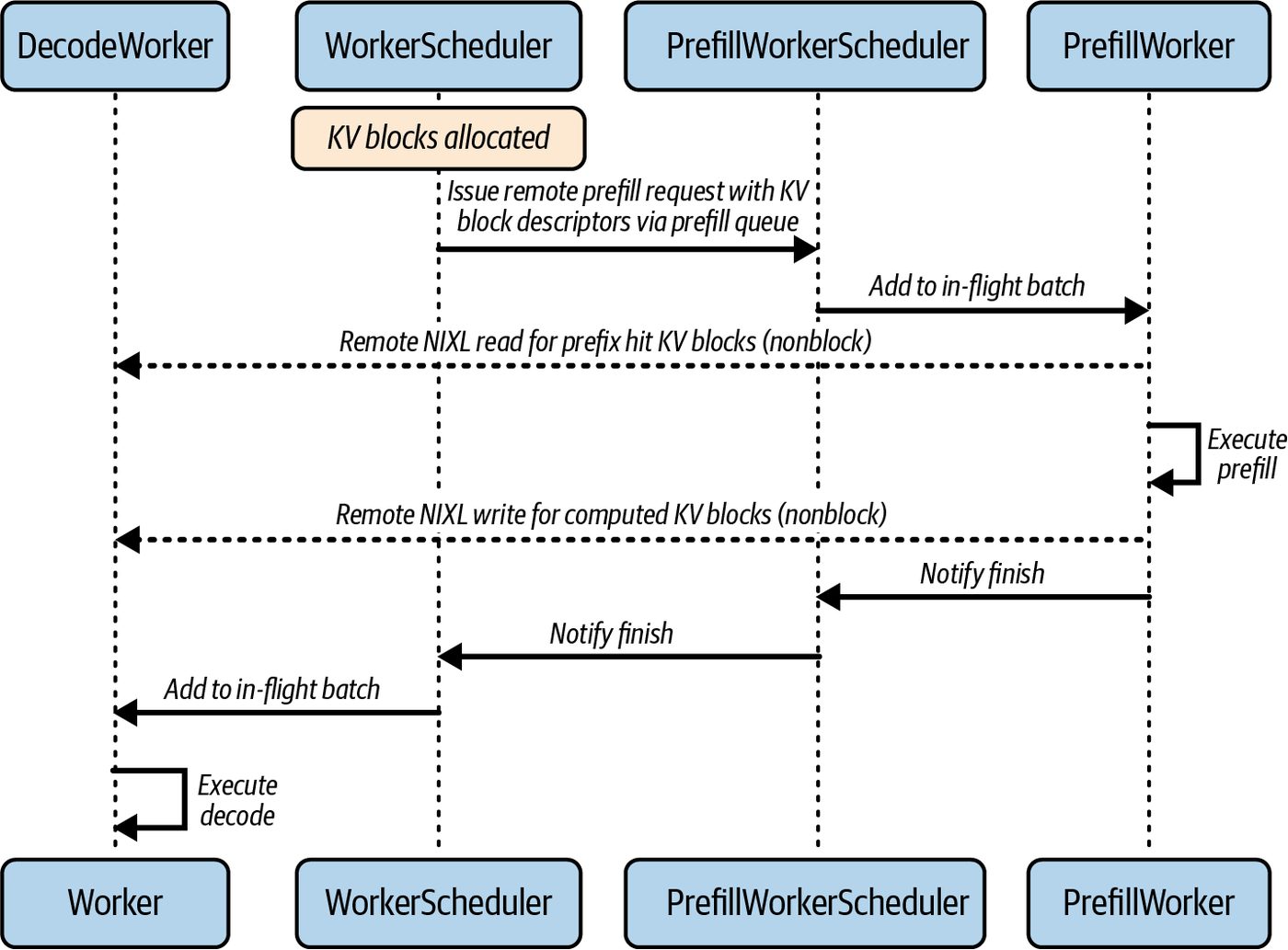
worker’s scheduler adds a corresponding decode request to its own decode pipeline.
This allows compute and data movement to overlap seamlessly. Make sure to use pre-
registered peer memory with large pinned window sizes to minimize re-registration
churn. You can verify zero-copy transfer overlap with the Nsight Systems timeline.
When validating end-to-end data movement and overlap, it’s recommended to profile
with Nsight Systems using trace flags. For InfiniBand link telemetry, add --nic-
metrics=true for HCA/NIC counters and --ib-switch-metrics-device=<GUIDs>
for switch counters. These will capture switch metrics and sample host/device activ‐
ity. Together, this will produce correlated CUDA kernels, UCX activity, storage met‐
rics, and network behavior. Following is a unified command that enables
CUDA/UCX tracing and collects CPU activity, GPU metrics, storage metrics, and
InfiniBand switch telemetry:
      nsys profile --trace=cuda-hw,osrt,nvtx,ucx,gds \
        --trace-fork-before-exec=true \
        --cuda-event-trace=true \
        --cuda-graph-trace=node \
        --cuda-memory-usage=true \
        --sample=cpu \
        --gpu-metrics-device=all \
        --nic-metrics=true \
        --ib-switch-metrics-device=<GUIDs> \
        --storage-metrics --storage-devices=all \
        --gds-metrics=driver \
        -o nsys_reports/prefill_decode \
        <your_launch_here>
                     It’s possible that the prefill and decode engines use different paral‐
                     lelism (e.g., tensor‐parallel) layouts. In this case, the system can
                     insert a layout transform kernel on the receiver side—after the
                     NIXL read (and before the data is used) to realign each KV block to
                     the layout expected by the decode worker.
Continuous batching. Decode servers rely heavily on continuous batching, also known as iteration-level batching. Unlike the prefill phase, which performs large matrixmatrix computations, the decoding phase performs many small computations since each new token generation is a relatively small vector-matrix computation since the individual token is represented as a vector. To avoid low GPU utilization for small, per-token workloads, decode workers can batch together multiple input sequences to create larger matrix-matrix computations (e.g., multiple token generations) at each iteration. This increases the arithmetic intensity for each decode task.
774 | Chapter 17: Scaling Disaggregated Prefill and Decode for Inference
For example, suppose 32 different text-generation requests are mid-stream and ready to generate their next token. Instead of computing 32 separate, single-token forward passes, a continuous batching scheduler will combine the requests and perform one forward pass that generates 32 tokens (one per sequence) in parallel. This way, matrix multiplications see an effective batch size of 32, which keeps the GPU compute units busy. The challenge is that not all sequences request a token at the exact same time. Some may finish early, and others may start late. Remember that you can batch across different requests and users. Most modern inference servers will automatically group decode steps from different users’ requests if the sequences have the same context length at that moment. This effectively per‐ forms batched decoding on the fly. Consider such solutions for maximizing decode throughput.
               In vLLM, CUDA Graph capture coverage is controlled by the flag
               called --max-seq-len-to-capture. Capture sizes are typically
               aligned to the maximum number of sequences. When a sequence
               exceeds this length, vLLM falls back to eager mode. It’s important
               to note that this flag does not control how many sequences are
               batched at runtime. The number of concurrent decode slots is con‐
               trolled by --max-num-seqs (upper bound on sequences in an itera‐
               tion). Set this explicitly for predictable memory use along with
               --max-num-batched-tokens.
Continuous batching addresses the issue of sequences requesting tokens at different times by dynamically updating the batch size at each step. Specifically, at each step, a continuous batching strategy will gather all sequences that are ready for a next token at that moment and batch them into a single decode step. If new requests finish prefill and become ready while the decode is in progress, they will join the next batch without waiting an arbitrary long idle period. This is in con‐ trast to static batching, which will wait to gather a full batch before decoding. If a sequence finishes by hitting an end-of-text token or a sequence-length limit, it is removed from subsequent batches immediately. If a sequence is not yet ready—per‐ haps it’s a long prompt still being processed in prefill—it won’t be included until it becomes ready. Effectively, with continuous batching, the batch size on each iteration can fluctuate. However, the server is always trying to maximize the batch size to include whatever sequences are available at that time—up to a limit. This achieves high utilization while minimizing per-token waiting time. Continuous batching makes sure that decode GPU workers never sit idle. They are always working on available requests. This maximizes their throughput under latency
Why Prefill-Decode Disaggregation? | 775
constraints by keeping the GPU busy—even as individual sequences await new tokens. Similarly, Microsoft’s DeepSpeed and NVIDIA’s TensorRT-LLM inference engines implement continuous or in-flight batching with paged KV caches to keep GPU uti‐ lization high during decoding. Specifically, DeepSpeed combines multiple generation requests, and TensorRT-LLM uses a scheduler to group decoding tasks across streams. In a disaggregated decode cluster, continuous batching becomes even more powerful. Since decode GPUs handle only generation, they can devote 100% of their cycles to this continuous loop without ever being interrupted by a large, bespoke prompt task. This leads to smoother throughput metrics—especially under load. Under high load, a decode node might have tens or hundreds of sequences concur‐ rently active. It can batch a large number of them at each iteration. This will maxi‐ mize hardware utilization. And under low load, even if only one sequence is active, the decode worker can immediately generate the token. It doesn’t have to wait to fill a batch. In this case, the GPU will be underutilized for that moment, but the latency for that single sequence remains low. As such, continuous batching handles both extremes: at high concur‐ rency it’s efficient, and at low concurrency it’s responsive. This is a good balance of high throughput and low latency.
Grouping variable-length sequences. Handling variable-length sequences in LLM infer‐ ence requires careful scheduling and batching to avoid wasted computation and memory. Mixing short and long prompts in one batch leads to padding overhead— sometimes up to 50% padding relative to the number of tokens. This wastes scarce GPU and network resources. When you batch prompts of differing lengths together, every shorter sequence must be padded to match the longest one. This padding introduces “no-op” tokens that still consume GPU cycles, memory bandwidth, and inter-GPU or network transfers. In some cases, padding can account for up to half of all tokens in common generative AI workloads. This significantly reduces inference efficiency. A straightforward solution is to group requests into buckets based on sequence length. This way, each batch contains sequences of similar sizes. Using static-length buckets like 0–512 tokens, 513–1,024 tokens, etc., fixes the batch boundaries and minimizes padding overhead. vLLM’s decode scheduler maintains a rotating pool of SequenceGroup instances (each prompt is a SequenceGroup). The scheduler advances each group after a fixed token budget per decode iteration. As soon as a SequenceGroup is done processing its chunk, it leaves the pool, and a new SequenceGroup joins the pool. This keeps the
776 | Chapter 17: Scaling Disaggregated Prefill and Decode for Inference
pipeline continuously full of work—without relying on static padding buckets or underutilizing GPUs. These batching and scheduling techniques align well with disaggregated prefilldecode deployments with separate prefill and decode clusters. Using this deployment configuration, the separate decode nodes can use techniques like continuous batching to minimize TPOT variance under strict SLOs. Meanwhile, the dedicated prefill nodes can be tuned independently for maximum input-processing throughput and minimum TPOT. NVIDIA’s Programmatic Dependent Launch (PDL) and device-initiated CUDA Graph Launch (discussed in Chapter 12) are used to reduce per-token launch over‐ head, overlap work, and eliminate bubbles between decode iterations. These features are generally enabled through the framework rather than manually in application code. When using device-launched graphs, instantiate with cudaGraphInstantiateFlagDe viceLaunch and keep nodes on a single device. Use PDL to overlap dependent kernels at the end of a step (e.g., decode iteration). This further trims per-token launch bubbles. By combining length-bucketing, continuous batching, disaggregation, PDL, and device-initiated CUDA Graphs, modern inference systems like vLLM, SGLang, and NVIDIA Dynamo can achieve both high throughput and low latency—even for wildly varying prompt lengths. And they do this without impacting resource effi‐ ciency or scalability.
               In vLLM, --max-seq-len-to-capture controls the maximum
               sequence length covered by CUDA Graphs. By default, this value is
               set to 8192. In continuous batching, vLLM may pad to the nearest
               captured size, so align --max-num-seqs and --max-num-batched-
               tokens to minimize padding waste. CUDA Graphs help to mini‐
               mize repeated CUDA-graph rebuilds for common sequence
               lengths. It does not directly dictate runtime batching behavior.
               Runtime batching in vLLM is managed by its decode scheduler’s
               dynamic SequenceGroup pool, as described previously. In produc‐
               tion, it’s recommended to tune --max-num-seqs and --max-num-
               batched-tokens alongside --max-seq-len-to-capture to bound
               HBM (KV) usage and reduce padding under continuous batching.
Memory management for the KV cache. Because decoding involves attending to the entire sequence seen so far—including previously decoded tokens—KV cache mem‐ ory is a critical resource for decode workers. Each sequence stores key and value
Why Prefill-Decode Disaggregation? | 777
tensors for each transformer layer—and each past token. Figure 17-5 shows an exam‐ ple KV cache being shared across different requests.
Figure 17-5. Managing and reusing KV cache data between requests
For large models and long sequences, KV memory grows linearly with tokens and depends on attention layout and dtype. A practical estimate is bytes_per_token = 2 x n_layers x n_kv_heads x head_dim x bytes_per_element. (Note: the 2 x accounts for keys and values per token per layer.) Consider a Llama-class 13B model with 40 layers, 40 attention heads (head dimen‐ sion is 128), and FP16. For a 4,096-token context with standard multi-headed atten‐ tion (MHA), the KV size is ~0.819 MB/token or ~3.36 GB total. With FP8 KV, that becomes ~1.68 GB. With grouped-query attention (GQA) with 8 query groups (n_kv_heads = 8), the 4,096-token KV is ~0.671 GB at FP16 and ~0.336 GB at FP8. And for multi-query attention (MQA) with 1 kv head, it is ~0.084 GB at FP16.
                     Make sure to always compute using the model’s actual n_layers,
                     n_kv_heads, head_dim, and KV precision since FP8 and FP4
                     change the bytes_per_element.
A GPU serving many concurrent sequences can quickly approach its memory limits purely due to KV cache storage—in addition to the model weights. As such, make sure your decode workers use such an optimized memory allocator to prevent GPU memory exhaustion when many long sequences are in flight. The following are strategies that decode workers use to manage KV memory efficiently:
778 | Chapter 17: Scaling Disaggregated Prefill and Decode for Inference
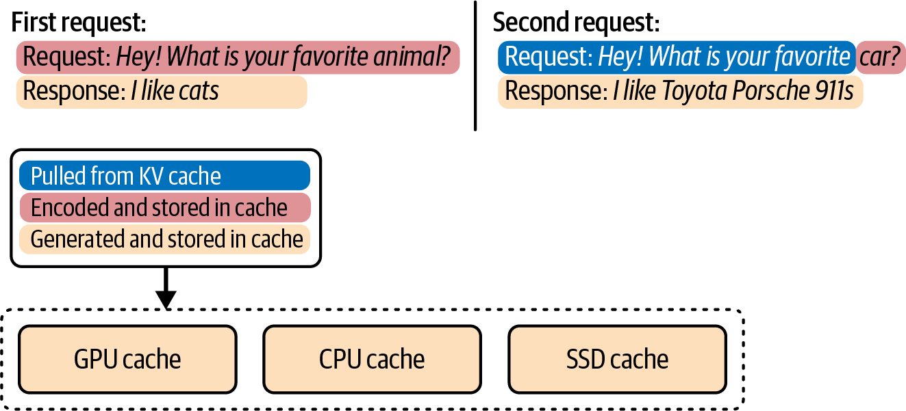
Paged GPU memory allocator
    vLLM’s PagedAttention mechanism is a prime example—it partitions the KV
    cache into fixed-size pages and can swap inactive pages to CPU memory. In addi‐
    tion to vLLM, paged KV memory managers are implemented in SGLang and
    NVIDIA TensorRT-LLM. NVIDIA Dynamo builds on these techniques. These
    systems also layer external KV tiers using DRAM and NVMe. And they can
    schedule recomputation versus I/O to balance bandwidth. This is common in
    projects like LMCache and other similar libraries and runtimes.
High-memory GPUs and custom allocators
    Decode servers often use GPUs with large HBM capacity (e.g., Blackwell B200’s
    180 GB HBM and Blackwell B300’s 288 GB HBM) to store the KV cache. Addi‐
    tionally, systems like vLLM and NVIDIA TensorRT-LLM use optimized memory
    managers that allocate KV memory in fixed-size pages to reduce fragmentation,
    enable efficient prefix reuse across requests, and manage hundreds of sequences
    of varying lengths. This efficiently shares memory without causing excessive
    fragmentation and waste.
KV cache offloading (e.g., paging out)
   When GPU memory fills up, the decode workers can offload older KV blocks to
   CPU RAM or colder storage such as NVMe. For instance, if a sequence generates
   1,000 tokens, but not all of them are currently needed right away, some earlier
   tokens’ KV can be moved to host CPU memory.
    When they’re needed, they can be brought back into GPU memory on demand.
    Offloading introduces a bit of a latency penalty when the tokens are needed for
    attention, so you should be careful when using offload. Decode servers often try
    to prefetch or overlap data transfer so that paging in KV data won’t impact gener‐
    ation as much.
Context limits and compression
   Some deployments impose a hard limit on the number of decoded tokens, or
   output sequence length. This is an application-level trade-off that caps the KV
   cache size and avoids unbounded growth. KV compression can also reduce KV
   memory required per token. For instance, storing KV at lower precision (FP16,
   FP8, INT8) can greatly reduce the memory usage.
    Another example is using multiquery attention (MQA), in which heads share a
    KV vector per token. This reduces the KV size proportional to the number of
    heads. This is a model architecture change that directly lowers the KV footprint.
    Grouped query attention (GQA) and DeepSeek’s Multi-Latent Attention (MLA)
    also help reduce the size of the KV cache.
Why Prefill-Decode Disaggregation? | 779
Memory hierarchy in disaggregation
   Another advantage of the disaggregated design is that the decode cluster’s GPU
   memory is fully dedicated to storing model weights + KV cache. It’s also not try‐
   ing to handle large prompt prefill computations, which, on a monolithic serving
   system, would consume a lot of extra memory temporarily during prefill.
      Each decode GPU typically loads the full model weights—unless using model
      parallelism—and then uses the remaining memory for KV storage. For instance,
      if model weights take 70 GB of a GPU’s memory and the GPU has 180 GB total,
      about 122 GB is left for KV.
      This directly impacts roughly how many tokens × sequences can be in-flight on
      that GPU. Disaggregation doesn’t eliminate KV memory issues, but by separating
      roles, you can choose decode node types that optimize for memory capacity and
      memory bandwidth.
      With the cluster configured this way, you need to decide when to offload a prefill
      to the prefill worker pool—or when to do it locally on the decode worker. Off‐
      loading has overhead, including queueing delays, network transfers, etc. As such,
      it should be used only when it will actually help latency. The decision is made by
      a routing policy, described next.
Disaggregated Routing and Scheduling Policies Not every request needs to be offloaded to a prefill worker. In fact, doing so when unnecessary would add overhead and not a lot of benefit. As such, a disaggregated inference system uses a routing policy to conditionally disaggregate and use the remote prefill path only when it is likely to help. Table 17-1 shows a high-level sum‐ mary of routing strategies, including KV-aware and prefix-aware routing.
Table 17-1. High-level routing strategies, including prefix-aware and KV-aware routing Routing strategy Description Round robin Routes to each node one by one Least requests Routes to the worker with the fewest active requests Prefix aware Uses the request’s prefix to select a worker KV aware Routes to the worker whose KV cache best matches the request
780 | Chapter 17: Scaling Disaggregated Prefill and Decode for Inference
The disaggregated router runs for each new request on the decode worker that ini‐ tially receives the request. And it makes a quick decision to either prefill locally or prefill remotely on the prefill worker pool.
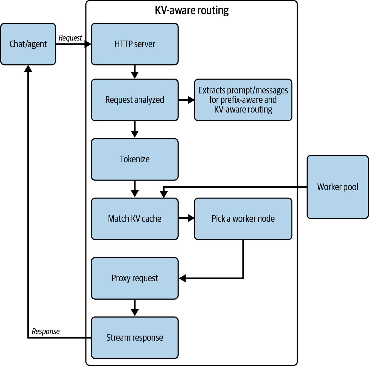
Routing factors The decision to offload prefill to the prefill worker pool can be based on several fac‐ tors related to the request and the system state. Common routing factors include cur‐ rent queue lengths, GPU memory availability, and even specialization since certain GPUs are better for certain models or prompt types. Advanced routers like vLLM’s KV cache-aware router also consider cache locality. They will route a request to a decode worker that already holds some of its prefix in cache. Figure 17-6 shows how an example KV-cache-aware router moves a request through the system based on data received from KV cache events emitted by the workers. The goal is to route in a way that maximizes cache hits and balances load. Table 17-2 summarizes some key factors that influence the routing decision in a typical disaggre‐ gated design.
Table 17-2. Factors influencing the router’s decision to offload a prefill Factor Description Effect on routing decision Prompt Number of tokens in the input Long prompts ⇒ more compute → offload prefill if length exceeds length prompt (after any prefix caching). threshold. Short prompts ⇒ do locally. Prefix cacheExtent of prompt already in the Large prefix cache hit (most of prompt cached) ⇒ prefill is effectively hit decode worker’s KV cache (from shorter and more memory bound → do locally. If no cache hits (all new previous requests). tokens) ⇒ heavy compute → offload likely beneficial. Prefill Number of pending tasks in the If the queue is long (prefill workers lagging) ⇒ avoid offloading new queue global prefill queue (how busy requests (do locally). If the queue is empty or light ⇒ prefill workers have length the prefill workers are). capacity → offload if other conditions are met. Decode Current load on the local decode If the decode GPU is busy with many decode streams, offloading helps worker load worker (ongoing decode tasks, parallelism (freeing up the GPU from heavy compute). If decode is mostly etc.). idle and the prefill queue is backed up, do local prefill to use available capacity. Latency SLO Priority or tightness of the Urgent low-latency requirement ⇒ might offload to ensure prompt is urgency request’s latency requirement. computed ASAP (especially if local decode is busy). Relaxed requirements might just run locally to save resources (see “QoS and early rejection policies” on page 792).
Why Prefill-Decode Disaggregation? | 781
Figure 17-6. KV-cache-aware request routing based on data received from KV cache events emitted by the workers
These factors will prefer to offload only requests that will benefit from the remote execution. These include long and compute-heavy prompts. Meanwhile, short and cache-hitting prompts are handled locally to minimize overhead. The thresholds are tunable. Each factor in Table 17-2 addresses a particular trade-off, as described next: Prompt length We don’t want to waste time offloading trivial prompts. The overhead of remote execution, even if small, isn’t worth it for a five-token prompt, for instance, since the decode GPU can handle that quickly on its own. Offloading is reserved for heavy prompts in which the decode GPU would otherwise be tied up for a long time.
782 | Chapter 17: Scaling Disaggregated Prefill and Decode for Inference
Prefix cache
    Modern inference systems often implement a KV cache that can store the KV
    pairs for previously seen context, such as earlier turns of a conversation or
    repeated boilerplate system prompts. If a new request’s prompt has a long prefix
    that overlaps with a prompt that has already been processed, the decode worker
    may already have that prefix’s KV data in memory. In that case, it needs to com‐
    pute only the remainder of the prompt for the cache-miss portion.
    If the remaining part is short, the benefit of offloading is reduced. Also, if the
    entire prompt is already cached due to a complete prefix hit, then no prefill com‐
    putation is needed at all. The decode can proceed immediately using the cached
    state. The router takes this into account by effectively considering effective
    prompt length = (prompt_length – prefix_cached_length).
    A large prefix hit not only reduces compute needed but also means a lot of KV
    data would have to be transferred to a prefill worker and back, which is pointless.
    Hence, such requests are kept local and leverage the cache.
Prefill queue length
    This essentially measures the load of the prefill worker cluster. If the prefill work‐
    ers are overwhelmed with many tasks waiting, sending yet another task their way
    could hurt TTFT more than it helps since the request would just sit in the queue.
    In those cases, decode workers are instructed to temporarily do more work
    themselves.
    This creates a natural load-shedding mechanism for the prefill cluster since the
    system gracefully degrades back toward local computation when the dedicated
    prefill tier is at capacity. When the prefill queue is short again and workers are
    caught up, offloading resumes for long prompts. This dynamic equilibrium is one
    reason disaggregation performs well across a variety of conditions.
Decode worker load
   While not always explicitly coded as such, the router inherently helps distribute
   the workload. If a decode worker is already busy decoding many streams, it can
   still offload new incoming prompts. This is good, as, otherwise, that GPU would
   have to juggle heavy compute and decoding concurrently—possibly slowing
   down both.
    Conversely, if decode GPUs are free because the system is very lightly loaded,
    they could handle longer prefills locally. In practice, an idle decode GPU is also
    likely to have an empty prefill queue since the overall load is low. The conditions
    already cover this case indirectly. But some implementations might include a
    direct check on local GPU utilization to decide whether prefill-offload is needed
    or not.
Why Prefill-Decode Disaggregation? | 783
Latency SLO and priority
    In systems with mixed SLAs or priority classes, the routing can be modified to
    improve QoS. For a high-priority request that must have the fastest TTFT, one
    might bypass queue checks and immediately offload so that it starts computing
    immediately—even if the decode GPU is free. In this case, the system can reserve
    that decode worker for a different high-priority decode task.
      Alternatively, if a request is low priority, the system might choose not to use pre‐
      fill cluster resources at all. Instead, it will just let it happen locally on the decode
      worker—or even delay it. We revisit priority request handling in “QoS and early
      rejection policies” on page 792, but just know that the basic router can be exten‐
      ded with these types of considerations.
The specific threshold values and weights used in the routing policy should be deter‐
mined empirically. For instance, you might find that prompts under 50 tokens are
faster to compute locally on a given type of GPU (e.g., Blackwell B200), whereas
larger prompts benefit from offload.
As new hardware is released, the thresholds might change since newer GPUs have
higher FLOPS and more memory bandwidth. As such, the break-even prompt length
for offload might become a bit higher since a single B200 can handle more tokens
fully on the decode worker, for instance.
                     You   should empirically adjust thresholds like PREFILL_
                     LENGTH_THRESHOLD when upgrading hardware due to improve‐
                     ments in compute FLOPS and memory bandwidth.
The outcome of effective routing is that the system achieves the best of both worlds. Short prompts are faster TTFT due to running locally—and they incur no extra over‐ head. Longer prompts get the benefits of parallelism since prefill and decode happen in parallel on different GPUs. Also, the prefill worker pool is utilized only when needed—and it avoids getting flooded when it can’t keep up. This type of conditional strategy was crucial in the DistServe prototype and in modern inference servers like vLLM and Dynamo. This allows them to improve use‐ ful throughput under latency constraints (goodput) rather than just raw throughput.
Example dynamic routing policy in code
In practice, the routing policy can be implemented as a simple conditional check. The
code here shows a simplified version of this routing logic:
      # Offload prefill decision running on a decode worker
      # (B200/B300 tuned)
      def should_offload_prefill(prompt_length: int,
784 | Chapter 17: Scaling Disaggregated Prefill and Decode for Inference
                               prefix_cached_length: int,
                               prefill_queue_size: int,
                               decode_active_reqs: int,
                               ttft_slo_ms: int = 500) -> bool:
        # Effective prefill after prefix KV hits
        eff_len = max(0, prompt_length - prefix_cached_length)
        # Tunables (kept in config; shown here for clarity)
        PREFILL_LENGTH_THRESHOLD = 256 # see split_policy.prompt_length_threshold
        PREFILL_QUEUE_MAX        = 10   # see autoscale/prefill queue-length guidance
        DECODE_LOAD_THRESHOLD    = 8    # active decode streams
        long_prefill = (eff_len >= PREFILL_LENGTH_THRESHOLD)
        prefill_available = (prefill_queue_size < PREFILL_QUEUE_MAX)
        # Prefer remote when prefill is compute-heavy
        # and the pool has capacity.
        if long_prefill and prefill_available:
            return True
        # If local decode is busy and prefill is moderately long,
        # free decode via offload.
        if decode_active_reqs >= DECODE_LOAD_THRESHOLD and eff_len >= 64:
            return True
        # Otherwise keep prefill local
        # (lower overhead / better cache locality).
        return False
In this pseudo-code, PREFILL_LENGTH_THRESHOLD is a system-tuned parameter, such as 50 or 100 tokens, that defines what counts as a “long” prompt. PREFILL_QUEUE_MAX is a threshold beyond which the prefill worker pool is considered saturated, specifi‐ cally if there are too many outstanding tasks. The decode worker calls should_offload_prefill() as soon as it receives a new request. If the function returns True, the decode worker will package the prompt into a message and push it onto the global prefill task queue. It then performs other work while waiting for the KV cache result to return. If should_offload_prefill() returns False, the decode worker immediately per‐ forms the prefill computation itself. This way, if prefill workers start lagging behind, new requests will fall back to local computation to avoid queuing delays. It’s a form of adaptive routing that balances the load between decode and prefill pools.
Example dynamic routing policy configuration In a production deployment, the routing policy should be configured through a file or UI rather than hard-coded. For instance, NVIDIA’s Dynamo allows specifying complex routing and autoscaling rules in a JSON or YAML config. Here is a simpli‐ fied example of a Dynamo Planner JSON that encapsulates some of the policy logic:
Why Prefill-Decode Disaggregation? | 785
      model: ...
      split_policy:
        prompt_length_threshold: 256
        prefix_cache_weight: 10.0
        queue_length_weight: 1.5
        decode_load_weight: 0.5
        enable_hotspot_prevention: true
      cache:
        reuse_prefix: true
        min_cache_hit_ratio: 0.75
      autoscale:
        prefill:
          min_replicas: 4
          max_replicas: 12
          scale_up:    { queue_length: 8, gpu_utilization: 80 }
          scale_down: { queue_length: 2, gpu_utilization: 40 }
        decode:
           min_replicas: 8
           max_replicas: 24
           scale_up:   { queue_length: 16, kv_cache_usage: 75 }
           scale_down: { queue_length: 4, kv_cache_usage: 30 }
      qos:
        enable_early_rejection: true
        low_priority_threshold_ms: 500
        reject_on_slo_violation: true
Here, the configuration defines a split_policy with a prompt_length_threshold of 256 tokens. It also specifies weights for factors like cache hit, queue length, decode load, and others. It also configures autoscale behavior for both prefill and decode roles, including how to scale up or down based on queue lengths, GPU utilization, and KV cache usage. In addition, it can apply some QoS rules like early rejection and tune what threshold to consider a request “slow.” In practice, Dynamo’s router reads this JSON at startup—or fetches it dynamically—to dictate each routing decision for requests spread across the entire cluster.
Capacity-aware routing As mentioned in the previous section, NVIDIA Dynamo supports dynamic routing policy. An implementation of this dynamic routing capability is Dynamo GPU Plan‐ ner. The planner uses metrics like TTFT, TPOT, and the estimated cost of KV cache transfer to decide to modify routing—or even reallocate/scale phase-specific GPUs— to reduce bottlenecks and adapt to shifts in the workload. This allows the system to maintain high performance during heavy surges in demand, as shown in Figure 17-7.
786 | Chapter 17: Scaling Disaggregated Prefill and Decode for Inference
Figure 17-7. NVIDIA’s Dynamo GPU Planner decides how to handle incoming requests and allocate GPU workers to prefill and decode based on GPU utilization metrics
Why Prefill-Decode Disaggregation? | 787
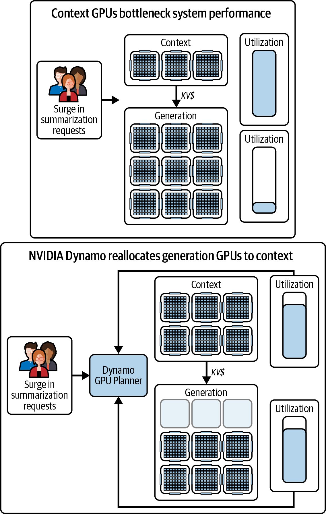
Here, Dynamo’s Planner chooses to shift more GPUs to the prefill (context) phase because of an influx of large summarization prompts that require a heavy amount of prefill (large inputs) relative to decode (small summary outputs). In contrast, if there is an influx of reasoning requests, the Planner can choose to real‐ locate GPUs to the decode phase since reasoning requests generate a lot of output tokens relative to the number of input tokens. In other cases, the Planner might choose to handle the request in a traditional monolithic fashion in which the prefill and decode happen on the same GPU worker node. In short, a component like NVIDIA’s Dynamo Planner can automate this decision process by constantly monitoring real-time metrics and comparing them to application-level SLOs like TTFT and TPOT latencies. Using this information, Dynamo Planner can dynamically determine whether to serve a request with full dis‐ aggregation, no disaggregation, or somewhere in between with more or fewer GPU resources allocated to each prefill/decode phase. The resulting adaptive system opti‐ mizes resource utilization across prefill and decode workloads—and meets aggressive performance targets.
Latency-aware routing The inference router can go beyond a simple threshold rule and use a more sophisti‐ cated latency score model to pick the best worker for each request. For instance, it might continuously compute a latency cost for each potential worker based on realtime metrics like how busy it is, how much memory is used, whether it has relevant cache, etc. It then sends the request to the worker with the lowest latency cost, for instance. Let’s assume that the worker with the lowest latency cost is the freest and most pref‐ erable worker. A simple latency cost function might be as shown here: # Lower cost is preferable latency_cost = 0.7 * (occupancy_percent) + 0.3 * (active_req_count) This particular latency cost function more heavily weighs the occupancy of the GPU. This correlates to how much work the GPU is currently doing. Secondarily, it corre‐ lates to how many requests are currently in flight on that engine. A new request would be sent to the engine with the lowest latency cost. The weights, 0.7 and 0.3 in this example, could be tuned based on empirical data. If KV memory usage is found to be a big predictor of slowdowns due to lots of data to swap or higher memory bandwidth usage, you would want to weigh it more heavily. A more advanced routing policy might include additional factors. For example, you can incorporate some of the following into your latency cost function:
788 | Chapter 17: Scaling Disaggregated Prefill and Decode for Inference
Exact cache match availability If a worker already has the needed prefix KV in its cache, a prefix hit, then it can serve the request much faster. In this case, the system can assign a large negative weight to reduce the latency cost and prefer this worker since lower is better in this scenario. KV occupancy Higher memory usage means the GPU is busier. In this case, the system assigns a positive weight to increase the latency cost and encourage the router to avoid this worker since lower is more preferable in this scenario. Active requests More parallel requests mean potential context-switching overhead, so this adds to the latency cost, which avoids this worker. Memory bandwidth utilization If a GPU is currently using a lot of its memory bandwidth by handling many long sequences, for instance, adding more work will just slow things down. This would increase the latency cost and discourage the system from choosing this worker. Recent KV use If the exact prefix was used recently on a worker engine—and the cache is “warm”—this will likely improve performance since the KV is still in an L2 cache or currently on its way from a prefill worker. In this case, you might include a small negative weight to reduce the latency cost and prefer this worker since it recently saw the prefix. Table 17-3 summarizes this type of advanced routing policy configuration. It lists some factors and example costs.
Table 17-3. Routing factors and relative costs Factor Interpretation Impact on latency cost KV occupancy (%) Higher = more memory pressure +3 (occupancy_percent) Active requests count More in flight = potential queuing +1 (active_req_count) KV cache match Engine already has the needed prefix KV –10 (large negative) (cache_match_flag) Memory bandwidth % High = memory bus is busy +0.5 (mem_bw_percent) Recent KV use Prefix was used on this engine recently –1 (recent_prefix_flag)
Why Prefill-Decode Disaggregation? | 789
Let’s modify the latency cost calculation with these additional metrics. The router
now calculates a composite latency cost, as shown here:
      # Lower cost is preferable
      def latency_cost(occupancy_percent: float,
                       active_reqs: int,
                       cache_match_flag: bool,
                       mem_bw_percent: float,
                       recent_prefix_flag: bool) -> float:
          return (
              3.0 * occupancy_percent
            + 1.0 * active_reqs
            - 10.0 * int(cache_match_flag)
            + 0.5 * mem_bw_percent
            - 1.0 * int(recent_prefix_flag)
          )
Prefill and decode clusters might even use slightly different formulas. For prefill, a
cache hit (e.g., prefix already computed) might be even more valuable to factor in,
whereas for decoding, memory bandwidth or available KV space might dominate the
decision.
The router needs telemetry from each worker. This includes metrics like its waiting
queue length, KV cache usage, memory utilization, etc., so that the latency cost can
be updated continuously.
The outcome is that the system can dynamically route traffic to where it will have the
least impact on latency. Under low load, all workers have low scores, and it may not
matter which one is chosen, as any worker can handle the request quickly.
Under high load, however, the router effectively load-balances by sending new work
to the workers that are most free. This will also take advantage of data locality (cache
hits) to reduce work. This reduces both average and tail latencies because work is less
likely to pile up behind busy engines when others are free.
Earlier, we saw how factoring in cache hits can cause the router to choose a slightly
busier server if it has relevant data cached. This results in faster service for that
request. The score function quantitatively captures this trade-off.
NVIDIA Dynamo performs a similar but opposite calculation in which higher is bet‐
ter. Specifically, it computes a remote prefill score, and if the score exceeds a thresh‐
old, it will offload to the prefill worker pool. Here is an example YAML snippet that
configures the system to use conditional disaggregation if the calculated score is
above a configurable remote_prefill_min_score value:
      disaggregated_router:
        enable: true
        policies:
          - metric: prefill_length               # Prompt length after prefix cache hit
            threshold: 256
790 | Chapter 17: Scaling Disaggregated Prefill and Decode for Inference
          action: prefer_remote    # if prompt > 256 tokens, offload prefill
          weight: 0.7
        - metric: prefill_queue_depth # requests queued for prefill workers
          threshold: 10
          action: prefer_local     # if queue > 10, lean toward prefill locally
          weight: 0.3
      remote_prefill_min_score: 0.5 # overall threshold decide remote prefill
Here, the router computes a score based on prefill_length and prefill_ queue_depth. In this case, if the prompt is longer than 256 tokens, it votes to pre fill_remote and offload the prefill. This part of the score calculation carries a weight of 0.7, as configured here. But if the prefill queue is very deep with more than 10 waiting tasks, as configured here, it will vote to prefill_local with a weight of 0.3, as configured here. If the combined score is greater than remote_prefill_min_score, or 0.5 in this case, Dynamo will offload the prefill. Otherwise, it will keep the prefill local and not off‐ load it.
Multipath inference (racing) Multipath inference, or sending the same request to two different model sizes or two different routes, is used for high reliability. It’s essentially racing to the fastest result and is often called racing. Google’s and Meta’s production systems are known to race models to reduce tail latency. It’s a costly but effective technique.
                If implementing multipath inference yourself, make sure your
                requests are idempotent and won’t cause issues if both paths exe‐
                cute. And make sure to cancel the slower path promptly to save
                GPU cycles.
Multibranch, parallel speculative decoding across workers As discussed in Chapter 15, some advanced inference servers support speculative decoding. Remember that speculative decoding generates multiple token branches in parallel, discarding those that are not the most ideal. While not a direct part of disaggregation, speculative decoding can be layered on top of the router’s decision-making process. For instance, the system could detect an uncertain speculative decoding branch and send multiple speculative requests to dif‐ ferent decode workers in parallel. This would generate multiple speculative nexttoken branches and mask the unpredictability in token-branch generation. This trades extra compute for lower latency for generations with unpredictable branches. If implemented, the router would coordinate these speculative efforts and then merge results. Resource usage would need to be bound to avoid overwhelming the cluster,
Why Prefill-Decode Disaggregation? | 791
but multipath inference is worth noting as a potential optimization for ultra-latencyaware inference, at the expense of additional, potentially wasted compute and memory-bandwidth cluster resources. In summary, a latency-aware router ensures each request is sent to the optimal place, considering both current load and potential speedups like cache reuse. It acts as the “brain” of a distributed serving system, working in concert with the lower-level scheduling on each GPU. Together with global scaling and KV caching strategies, it forms a comprehensive approach to maximize goodput and minimize latency.
QoS and early rejection policies QoS policies prioritize or throttle certain requests to meet latency targets. Early rejec‐ tion, also called admission control, can refuse low-priority queries when the system is saturated. This way, it preserves resources and SLOs, such as latency for other requests. Modern systems do this based on a queue time threshold. For example, if a request has sat in queue > X ms, it might be better to reject it or offload it to a lower-tier service rather than let it severely violate the SLO. This kind of QoS guard is increasingly common for mission-critical inference systems. In ultrascale inference systems, QoS mechanisms are needed to maintain tail latency guarantees under heavy load. Even with an optimized disaggregated cluster configu‐ ration, if load exceeds capacity, requests will start queuing and latencies will rise. Rather than allowing latency SLOs to be violated for all requests, a well-designed sys‐ tem will prefer to shed load gracefully. It can do this by rejecting or deferring some requests, especially lower-priority ones, when it is clear that serving them would break the latency guarantees for others. This is analogous to how web servers return HTTP 503 “overloaded” errors under extreme load. For LLM serving, we might proactively refuse or down-sample requests if we can’t guarantee serving them in time. Here are a few components to QoS in the context of prefill/decode disaggregation: Latency SLO tracking The system should be aware of target TTFT and TPOT goals. For instance, the first token must return within 200 ms 99% of the time. Using internal telemetry, each decode worker can estimate the current TTFT for a new request if it were to be accepted right now and based on current queue lengths, etc. It can similarly estimate TPOT if another decode stream is added. Admission control (early rejection) Before a request is fully accepted and assigned, the system can perform a check to see if admitting this request will overload the system or violate SLOs. If yes, it can
792 | Chapter 17: Scaling Disaggregated Prefill and Decode for Inference
    reject the request immediately with a “server busy, try later” type of response.
    This is called early rejection. In practice, you can use a global view of system load
    or simply a single node’s heuristic to trigger the early rejection.
    OpenAI’s public API, for instance, returns an error if the backlog is too high. It
    does this rather than violate the latency commitment. Some providers dynami‐
    cally lower the maximum generation length during peak load. This effectively
    trades off answer quality for latency.
Prioritization
    Not all requests are equal. Some requests might be high priority if they come
    from paying customers or critical services, for instance. Others might be lower if
    they’re from free-tier users or background jobs. The system can incorporate pri‐
    ority into scheduling decisions. For instance, a decode worker’s scheduler could
    serve high-priority decode tasks first. Or the prefill task queue could be ordered
    by priority. If things get busy, low-priority tasks may wait longer or be fast-failed
    in favor of high-priority ones.
Graceful degradation
    If the system starts to get overloaded, instead of outright rejecting requests, it
    could degrade service for less important ones. For instance, it might use smaller
    models for less important requests, truncate their prompts, or cap the number of
    output tokens. One simple approach is to temporarily reduce the maximum
    allowed prompt length or output length for lower-tier requests when load is high.
In the context of disaggregation, one interesting form of graceful degradation is to
temporarily disable remote prefilling for lower-priority requests when the system is
under stress. Since remote prefill uses additional cluster resources to optimize
latency, one could decide that low-priority queries should just do local prefill and use
only the decode worker resources. This would produce a slower response for these
requests, but it frees up the prefill workers for high-priority queries.
For instance, an inference server could tag each request with a priority and have the
router ignore the should_offload_prefill logic for low-priority requests when pre‐
fill workers are busy with high-priority tasks.
Here is an example of an early rejection policy. This could run on each decode worker
before processing a requestor even upstream on an LLM gateway:
    # Early rejection based on estimated latency and priority
    from dataclasses import dataclass
    class QoSController:
        def __init__(self, ttft_slo_ms: int = 500):
            self.ttft_slo_ms = ttft_slo_ms
def admit_request(self, priority: str) -> bool:
Why Prefill-Decode Disaggregation? | 793
                # The queue length and per-request averages are fed by the metrics system
                est_ttft = (get_current_prefill_queue_length()
                            * get_avg_prefill_time_per_req()
                            + get_current_decode_queue_length()
                            * get_avg_decode_time_per_req())
if est_ttft > self.ttft_slo_ms and priority.lower() == "low": # reject low priority request to protect SLOs return False return True Here, we estimate TTFT by looking at how many prefill tasks are queued since each will add some delay, as well as how many decode tasks are ahead. Note that decode tasks typically overlap, so this is a rough estimate. If the estimated TTFT exceeds the allowed maximum, the SLO, then for a low-priority request we reject it and return False from the should_offload_prefill function. For a high-priority request, we still accept it and perhaps sacrifice some other queued work, if necessary. A more sophisticated approach is to preempt a low-priority request that’s already queued to make room for the new high-priority one. This is often implemented by maintaining separate queues per priority level. Diving a bit deeper, in the preceding example, the avg_prefill_time_per_req() and avg_decode_time_per_req() functions compute the values on the fly using an expo‐ nential moving average of the observed per-request prefill and decode durations. They’re normalized by the number of prompt tokens (prefill) and generated tokens (decode). And for inputs of varying length, the engine extrapolates by multiplying these per-token averages by the actual token count for each request. The get_current_prefill_queue_length() and get_current_decode_queue_ length() functions retrieve the number of pending prefill and decode tasks tracked by the scheduler’s internal queues. These values are maintained by the scheduler. These per-token timing estimates are refreshed in real time using the scheduler loop, which, by default, updates every second from using /metrics endpoint. This captures dynamic workload changes. Early rejection and prioritization make sure that when the system nears saturation, it fails in a controlled manner rather than collapsing. Users with the most important requests continue to get served within the provided SLO. Meanwhile, less important traffic is shed. In many production deployments, implementing this requires coordination with the LLM gateway layer. Specifically, the gateway might return a specific error code or return a code indicating server-overload back to the client. The key is that the system keeps itself in a state where it can meet the latency promises for the work it does accept, rather than oversubscribing and missing SLOs for everyone.
794 | Chapter 17: Scaling Disaggregated Prefill and Decode for Inference
Another QoS consideration is adaptive generation limits. If the decode phase threat‐ ens to run too long and cause a TPOT SLO violation, the system might cut off the generation early. For instance, if a user requested 1,000 tokens but the system is under pressure, it might only allow 200 tokens to be generated and then stop. This leaves resources for other requests. QoS policies prioritize or throttle certain requests to meet latency targets; early rejection can refuse low-priority queries when the system is saturated to preserve SLA for others. In short, disaggregation reduces inherent interference, but load spikes can still over‐ whelm any fixed capacity. QoS mechanisms complement the disaggregation architec‐ ture by making sure it delivers on its latency promises. Early rejection will reject or deprioritize some work to protect the latency of the rest of the requests. When building ultrascale systems, these policies are as important as core perfor‐ mance optimizations. Without them, a flood of requests could ruin all attempts to improve performance by creating huge queues and slowdowns.
Scalability of Disaggregated Prefill and Decode Another aspect of scalability is how performance holds as more nodes are added. The disaggregated approach, by design, scales relatively linearly in many respects. You can add more prefill nodes to handle more prompt throughput. And you can add more decode nodes to handle more token-generation throughput. The main challenge is balancing them. Adaptive schedulers become even more important as scale increases. This is because the chance of an imbalance, such as a shifting traffic pattern, is much higher in a large system. A dynamic ratio configura‐ tion allows clusters to rebalance the ratio of prefill and decode on the fly. Another consideration is multimodel serving. Disaggregation allows you to share decode capacity between models if their decoding characteristics are similar. For instance, if model A and model B are hosted on the same cluster, you can dedicate some decode workers to handle both types of models. This is particularly useful when hosting different LoRA adapters that reuse the same base model architecture. This would give you a super flexible, multitenant, multimodel, prefill-decodedisaggregated inference server system. This is beyond our scope, but just know that disaggregation’s modularity gives you this type of flexibility. You can have a common decode pool for multiple models, each with its own prefill frontend. Finally, let’s analyze tail latency in very large systems. As ultrascale inference systems scale out to thousands and millions of GPU nodes, it becomes harder and harder to control tail latency. This is because with more servers, the chance that one fails is much higher.
Why Prefill-Decode Disaggregation? | 795
Disaggregation can help here, too. Isolating prefill tasks on one node and decode tasks on another means a slow node on one side won’t drastically impact tasks on the other side. Techniques like early rejection, two-level scheduling, and KV cache reuse, discussed in this chapter, can help to mitigate stragglers. For instance, caching large parts of a request’s context means that one slow operation won’t slow down the whole genera‐ tion as much—because a lot of the computation was already done. In summary, disaggregated systems are more robust at scale when properly config‐ ured and tuned. These systems can maintain consistent latency even as concurrent requests grow into the millions and billions. By removing one interference factor and adding adaptability, the tail latency distribution improves —or, at least, won’t degrade as fast with load.
Key Takeaways
The techniques covered in this chapter, from high-speed RDMA transfers of KV
cache to dynamic routing algorithms and QoS policies, have proven to be essential
components for large-scale production inference workloads. Here are the key
takeaways:
Eliminate prefill-decode interference to improve latency
    Separating prefill and decode phases removes interference and head-of-line
    blocking. This yields tighter latency distributions since long prompts won’t delay
    shorter prompts. This also lets each phase meet its latency SLO reliably.
Optimize each phase independently
    Prefill (prompt processing) is compute bound and benefits from maximum par‐
    allelism and high FLOPS. It prefers high-compute GPUs and techniques like
    FP8/FP4 reduced precision to minimize TTFT. Decode (token generation) is
    memory bound and benefits from high-memory bandwidth GPUs and tech‐
    niques like continuous batching to maximize throughput per token. Disaggrega‐
    tion allows different hardware and parallelism settings for each phase. A fixed,
    one-size-fits-all configuration does not allow this.
Leverage the KV cache
    It’s common to use a KV cache to avoid recomputing prompt prefills. A smart
    router can decide if a new request should be offloaded to a prefill worker or han‐
    dled directly on the decode worker. The routing policy should consider prompt
    length, cache hits, and cluster load.
796 | Chapter 17: Scaling Disaggregated Prefill and Decode for Inference
Route intelligently Modern inference servers like vLLM, SGLang, and NVIDIA Dynamo use a mul‐ tifactor scoring algorithm to route prefill and decode requests to maximize throughput and maintain adequate latency. Many frameworks also refer to TPOT as inter-token latency (ITL) in schedulers and dashboards. It’s recommended to track TTFT (p50/p95/p99) and ITL/TPOT (p50/p95/p99) separately for prefill versus decode nodes. This way, performance regressions are easier to debug dur‐ ing upgrades, for instance. For example, they will skip remote prefill if the prefill servers are saturated or if the prompt is short. Use QoS to maintain SLAs at scale Apply admission control and prioritization under heavy load. It’s best to fast-fail excess or low-priority requests than to let the system’s latency explode for every‐ one. Real-world systems implement early rejection by returning “busy” errors or a degraded response length—to guarantee that 99th-percentile latency stays under a given threshold. Disaggregation and QoS together prevent overload cascades—even in billion-request-per-day scenarios.
Conclusion Disaggregated prefill and decode is now common in modern high-scale LLM infer‐ ence. Virtually all major AI providers like Meta, Amazon, NVIDIA, Google, and OpenAI (or “MANGO”) have embraced some form of disaggregated architecture in their large-scale LLM deployments. While most of these companies do not publish their complete production architec‐ ture, there are numerous open source implementations (e.g., vLLM, SGLang, NVIDIA’s Dynamo) that demonstrate this approach and its benefits. Disaggregated PD produces higher goodput, or useful throughput under latency constraints, and better cost-efficiency than monolithic designs. In the next chapter, we’ll continue combining modern GPU and networking hard‐ ware with more advanced scheduling and caching optimizations to serve multitrillion-parameter model LLMs to billions of users without sacrificing latency or blowing up costs.
Conclusion | 797