Ch 16 — Profiling, Debugging, and Tuning Inference at Scale
Operating a large LLM inference cluster requires monitoring and debugging tools that make sure everything is running as expected. They also help you quickly identify bottlenecks when performance strays from its target. In this chapter, we demonstrate how to monitor and debug these complex systems using tools such as NVIDIA Nsight Systems for profiling and Prometheus/Grafana for cluster-wide telemetry. We also show how to collect and interpret key metrics like GPU utilization, memory pressure, tail latency percentiles, cache hit rates, per-token timing, and more. These help guide our inference engine performance optimizations. Next, we discuss operational performance tuning, including production-proven methods to optimize GPU utilization, reduce inference latency, and increase through‐ put in large clusters. This includes techniques for overlapping computation and com‐ munication, scheduling and batching requests, and using high-speed interconnects like NVLink, NVSwitch, and InfiniBand effectively. We’ll also compare techniques for real-time quantization for inference, including methods to compress models to 8-bit and 4-bit precision using implementations like Generalized Post-Training Quantization (GPTQ) and Activation-Aware Weight Quantization (AWQ). Along the way, we’ll discuss the trade-offs between weight-only quantization versus quantizing both weights and activations. We provide practical guidance on applying quantization in serving pipelines to reduce memory usage and increase throughput—all while preserving model accuracy. Finally, we consider application-level optimizations that complement low-level per‐ formance tuning. These include strategies like prompt compression, prefix caching, deduplication, query routing (e.g., fallback models), and partial-output streaming.
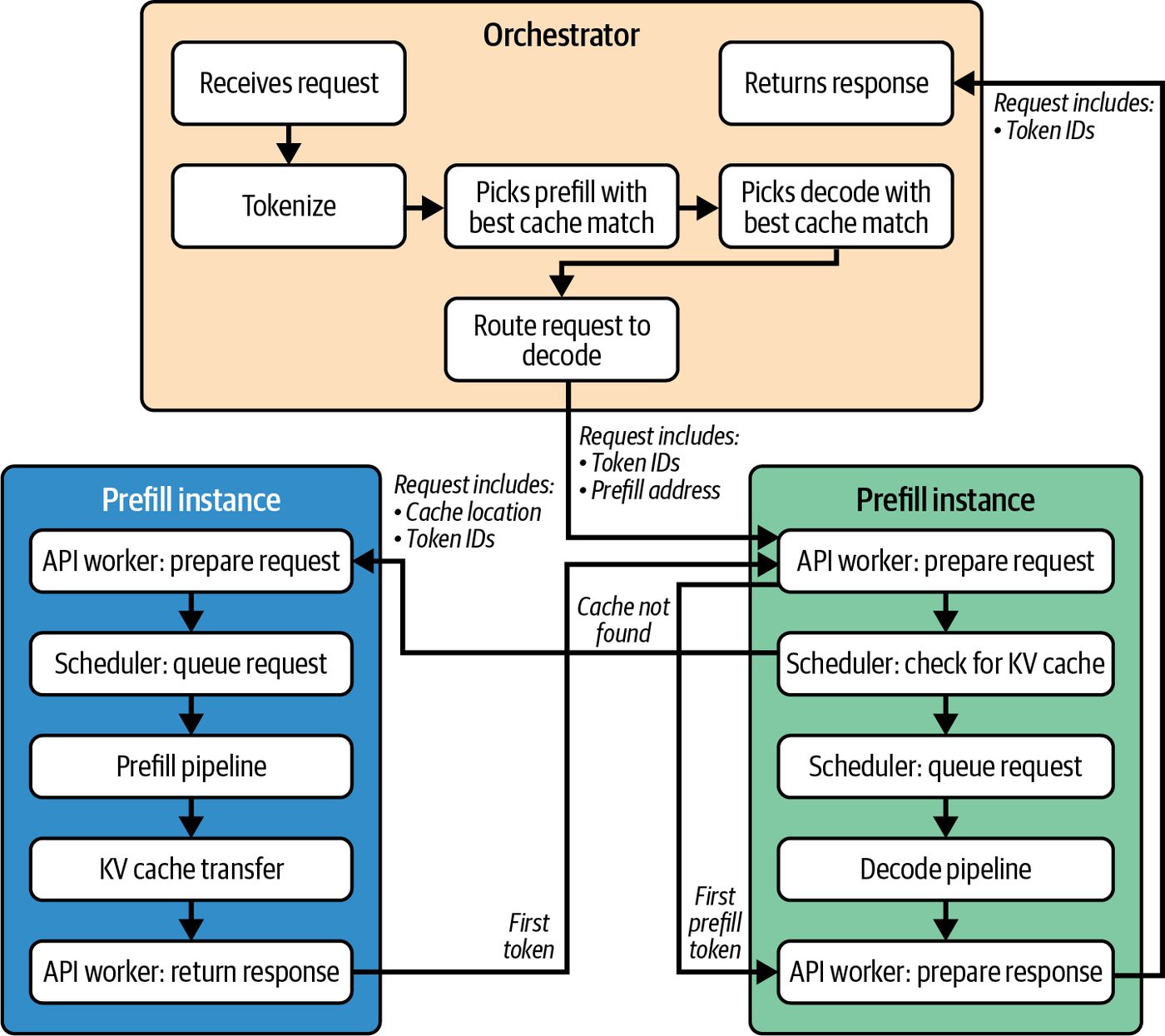
Profiling, Debugging, and Tuning Inference Performance There are a lot of moving parts in modern LLM inference engines—especially with disaggregated prefill and decode. The lifecycle of a typical request involves many components, as shown in Figure 16-1.
Figure 16-1. Lifecycle of a typical request in a disaggregated prefill and decode LLM inference system
Given such complexity, the workflow for tuning inference performance is very itera‐ tive. It requires careful tuning and continuous verification. First, you should observe metrics and identify the current bottleneck, including a GPU not fully utilized or higher-than-expected latency. Next, form a hypothesis for improvement, such as “increase the batch size” or “increase communicationcomputation overlap for operation X.” Then, implement a fix and test the hypothesis.
702 | Chapter 16: Profiling, Debugging, and Tuning Inference at Scale
Then, you should ideally test the fix in a staging environment with a representative workload using profiling tools to validate that the change behaves as expected. For instance, you can verify that an operation is demonstrating proper memory and com‐ pute overlap. Last, you should deploy the fix into production and monitor Grafana and the logs to validate that the fix improved throughput and latency on a real workload. Repeat this workflow as new bottlenecks appear. This observe-hypothesize-tune loop should be continuous. Modern deployments often automate these steps. For instance, you can use scheduled load tests—and sub‐ sequent anomaly detection on key metrics—to trigger a tuning workflow.
                It’s recommended to perform canary rollouts when deploying opti‐
                mizations to production, including updated inference runtimes
                and model variants. By deploying the optimization to a small sub‐
                set of traffic running on a small number of servers, you can validate
                the optimizations before full production deployment to all end
                users. This incremental approach helps reduce the “blast radius” of
                unexpected side effects by catching them early without impacting
                all users.
Consider a scenario in which host-side CPU utilization is spiking to 100% due to excessive tokenization or inference data preprocessing. This will limit how many con‐ current streams the inference engine can handle. One fix might be to move the pre‐ processing to the GPU using a GPU-accelerated tokenizer library or a custom GPU kernel written in CUDA or OpenAI’s Triton language. After deploying the new library or kernel, you should monitor CPU utilization before and after. If you see the CPU utilization decrease and overall throughput increase, then the system is no longer bottlenecked by the CPU-based input preprocessing. You should also pay attention to cache hit rates for any type of cache, including prefix cache, prompt-embedding cache, and KV cache. You should have metrics for “cache hits” versus “cache misses.” A high cache-hit rate means that the system is reusing data effectively. In contrast, if you see a high cache-miss rate, then you likely want to tune the cache size, eviction policy, or caching strategy to maximize cache hits. vLLM’s LMCache component allows adjusting the GPU versus CPU cache ratio. If misses are high due to GPU memory limits, you can enable its paged cache offload capability so that the CPU can help out. Always make sure your cache eviction policy (Least Recently Used [LRU], Least Frequently Used [LFU], etc.) aligns with the access patterns. Another scenario is using a KV cache to reuse data for identical input-sequence pre‐ fixes among batched requests to avoid recomputing the KV for the prefix. In this
Profiling, Debugging, and Tuning Inference Performance | 703
case, you want to measure how often requests share a prefix. This leads to a prefix merge event and increments the prefix cache hit metrics in vLLM including vllm:gpu_prefix_cache_queries and vllm:gpu_prefix_cache_hits. These let you compute the hit rate as hits per queries, for example. Measuring prefix-merge rates helps you correlate with actual cache‐hit rates to gauge the real benefit of your caching layer. This way, you can adjust batching and schedul‐ ing policies to maximize shared prefixes—and predict end‐to‐end throughput and latency improvements under different workloads. You can run synthetically generated data on the inference engine to test prompts with many repeated prefixes. Hopefully, you will see a reduction in prefill compute due to the prefix merging. Modern LLM inference engines like vLLM and SGLang expose prefix-merge metrics natively. But if prefix-merging is not a first-class metric exported by your inference engine, you should instrument a custom counter for “prefix deduplicated tokens” to monitor its effectiveness.
                     If you see that prefix merging is not performing as expected, you
                     should check if the prefix-matching logic is failing. Start the debug‐
                     ging process by checking if there are tokenizer differences. This is
                     the likely cause of most prefix-matching issues.
In addition to performance, monitoring helps with capacity planning. By tracking how utilization and latency behave as load increases, you can project at what point the system will hit a particular limit, such as p95 (95th percentile) latency starting to rise exponentially. In this case, the dynamic batch size might be increasing to a point of diminishing return.
                     If you are using a tiered caching strategy, including an NVMe-
                     based KV cache extension, make sure to monitor the I/O latency of
                     the device. High I/O latency will significantly decrease cache
                     performance.
When per-GPU concurrency reaches its limit and further batch-size increases no longer increase throughput, you may want to scale out by adding more GPUs, deploying additional model replicas, or increasing the number of experts to distribute work across more compute units. You should also consider model compression—or switching to lower precision (FP8/ FP4)—to get more effective throughput per GPU before scaling out. However, once hardware is saturated (e.g., SMs at 100% and memory bandwidth near peak
704 | Chapter 16: Profiling, Debugging, and Tuning Inference at Scale
utilization), adding more GPUs or using tensor/pipeline parallelism is likely the only path to higher throughput. And remember to always weigh the cost of new hardware against the efficiency gains. There are times when upgrading to newer GPUs with more memory and FLOPS will be more cost-effective than scaling out a fleet of older GPUs. Increasing the expert count can raise your throughput ceiling—but only if you also improve expert routing and scheduling to manage the extra all-to-all communication. Otherwise, naive scaling may simply shift the bottleneck to the network. Next, let’s discuss monitoring and how to verify that our optimization efforts are actually paying off.
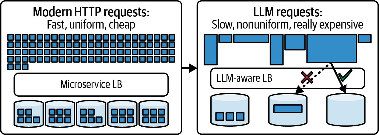
Monitoring System Metrics and Counters Unlike traditional microservice invocations, which are relatively uniform and pre‐ dictable in their execution time, LLM requests are nonuniform and can vary wildly in terms of latency. This difference is shown in Figure 16-2.
Figure 16-2. Difference between traditional microservice invocations and LLM invocations
For ongoing monitoring in production, it’s common to use Prometheus to collect metrics from each GPU compute node—as well as Grafana dashboards to visualize them. Key GPU metrics to track include GPU utilization (percent of time the SMs are busy), GPU memory usage, copy engine utilization, PCIe and NVLink throughput, and GPU temperature and power (e.g., throttling). Note: Low-level counters such as L1 and L2 activity, occupancy, and instruction throughput can be collected with Nsight Compute or CUPTI rather than DCGM and Prometheus.
               The cudaMemPool metrics and asynchronous allocator statistics are
               helpful when monitoring memory fragmentation. These should be
               integrated into your monitoring, as this will greatly facilitate
               debugging system performance issues in production.
Profiling, Debugging, and Tuning Inference Performance | 705
It’s also important to monitor interconnect utilization, including NVLink, NVSwitch bandwidth, and NIC throughput. This way, you will catch communication bottle‐ necks in multi-GPU and multinode cluster configurations. NVIDIA’s Data Center GPU Manager (DCGM) exposes many GPU metrics, which Prometheus can scrape and collect. For instance, DCGM provides DCGM_FI_DEV_GPU_UTIL for SM utilization %, DCGM_FI_DEV_MEM_COPY_UTIL for mem‐ ory copy engine utilization, and DCGM_FI_DEV_FB_USED for framebuffer memory used, among others. DCGM exposes NVLink error counters and can expose throughput counters on some platforms and driver versions. For sustained link utilization, also use nvidiasmi nvlink and Nsight tools. You should integrate these metrics into your dash‐ boards and set up alerts to help identify when the network is saturated with crossGPU and cross-node communication traffic. DCGM tracks Xid counters, as well as critical GPU errors.
                    While DCGM exposes NVLink counters, as of this writing, dcgm-
                    exporter does not expose per-link bandwidth on all platforms by
                    default. So if you need link-level throughput, you may need to
                    query DCGM directly or extend the exporter.
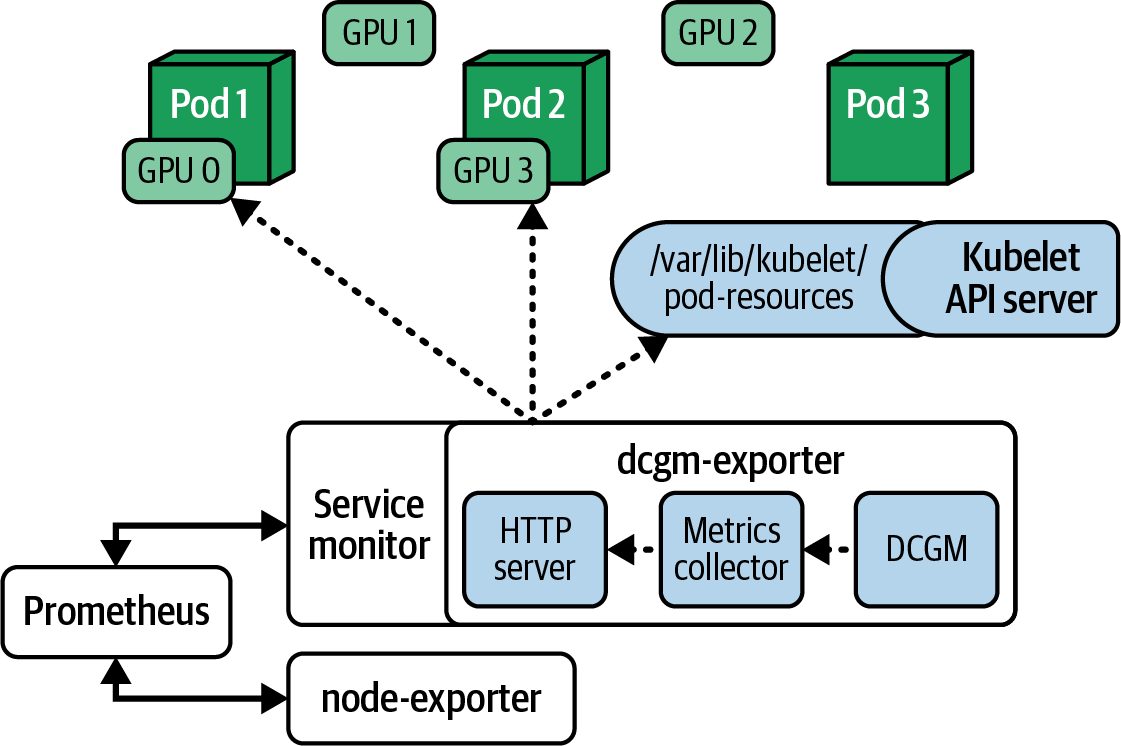
It’s also recommended to collect high-level application metrics like queries/requests per second, average latency and p95/p99 latency, number of active contexts, and throughput in tokens/sec. Metrics on KV cache utilization and size (overall and per node) are extremely important to monitor as well. You can set up Prometheus node exporters to gather all of these metrics from each node, collect the data in one place, and even set up alerts for critical thresholds. Gra‐ fana can then plot these metrics for real-time dashboards to share with your team. Figure 16-3 shows how the metrics are collected from each GPU in a Kubernetes cluster and exported to Prometheus to be visualized with Grafana, for example. This way, when you deploy a new optimization to increase batching, for instance, Grafana will immediately show if GPU utilization on each GPU increases. You can also monitor to make sure p95/p99 latencies stay within the target. Counters are extremely useful to measure as well—especially with dynamic and adap‐ tive systems. For instance, if your inference engine dynamically adapts the batch size to current conditions, you may want to increment a “batch size change” counter.
706 | Chapter 16: Profiling, Debugging, and Tuning Inference at Scale
Figure 16-3. DCGM collects metrics from the Kubernetes GPU nodes and sends them to Prometheus
The other option is to log the change in a logfile, but this would require a slow, textbased search/aggregation to analyze the logfile offline using Apache Spark, for instance. You would then need to manually correlate the result of the logfile analysis with the Prometheus metrics. By incrementing a simple counter for interesting application-level events (including errors), the data is pushed to Prometheus and instantly viewable in the Grafana dash‐ board alongside all of the other metrics in real time. In addition, consider using structured logging and distributed tracing for critical events. Modern application performance management (APM) tools—as well as OpenTelemetry—can ingest these logs/traces and correlate them with metrics. This provides a consistent timeline view of events across the entire system. Having insight into this timeline will help speed up the time it takes to debug performance issues. If you continuously monitor these metrics, you gain insight into where to tune next. For instance, if GPU utilization is below expected, you can check if GPU memory is maxed out or not. If it’s not fully utilized, you can try to increase the batch size or maximum number of concurrent requests. Make sure to keep an eye on latency service-level objectives (SLOs), however. You don’t want to exceed these.
               Modern inference servers expose a “maximum latency” setting for
               dynamic batching. Tune this to meet your SLOs. Increasing it raises
               the batch size (throughput). Increasing it too much will hurt p99
               latency. Continuously adjust this in light of your latency targets.
Profiling, Debugging, and Tuning Inference Performance | 707
In contrast, if GPU memory is near maximum, the inference engine might start swapping out inactive KV cache data to host CPU memory or NVMe storage. This will reduce GPU utilization, as the GPUs need to wait for the additional data transfers from slow CPU memory or disk.
                     If you see a spike in GPU memory copy-engine utilization—or
                     abnormal NVLink utilization that aligns with low SM utilization—
                     your inference engine is likely swapping KV cache data in and out
                     of GPU memory. This will bottleneck your system due to excessive
                     data transfer latency.
If you are swapping, you can adjust the inference engines’ paging parameters to reduce thrashing, apply FP8 or FP4 quantization, increase GPU memory allocation for cache, and potentially change the swapping strategy. This should bring copy uti‐ lization down and compute utilization up—exactly what you want to see. Grafana is also used for latency tracking. You can plot the distribution of end-to-end request latency—often measuring both prefill latency and per-token latency as well. If the p99 latency spikes at certain times, you should correlate it with GPU metrics and other logs. For instance, a p99 latency spike might correlate with a period when GPU utilization drops. Perhaps the latency spike correlates with a traffic surge that triggered a larger dynamic batch size. This could lead to higher latency for that period of time. To ver‐ ify, you can overlay RPS (requests per second) on the latency graph in the Grafana dashboard to see if the two charts correlate. If the spike was expected due to a dynamic increase in batch size per our hypothesis, make sure it isn’t exceeding your service-level agreement (SLA). If it is, you can try decreasing the maximum request-batch queue delay or reducing the maximum batch size to put a limit on the latency. Logs are invaluable when diagnosing issues as well. You should instrument the code to log key events such as when a batch is formed, when a communication starts/ends, etc. It’s best to use the DEBUG level so that you can enable/disable it as needed—and not impact request-response latency. When you enable debug logging, you’ll see a step-by-step timeline in text format. In one debugging session, it’s likely that you’ll use both the logging timeline and Prome‐ theus/Grafana metrics together. For instance, you can see how often an all-to-all communication takes longer than 5 ms. With the combination of log-based timeline and metrics, you can see outliers such as network issues that may have slowed down one iteration in the all-to-all communica‐ tion exchange. If this continues to happen, you can raise the expert capacity factor so
708 | Chapter 16: Profiling, Debugging, and Tuning Inference at Scale
that any excess tokens automatically spill over to a secondary expert replica—ideally hosted on a GPU with a more stable network path. This will balance the load and minimize the latency.
               In practice, setting the capacity factor to 1.2–1.5 is common, as this
               allows 20%–50% extra tokens to be reassigned when a primary
               expert is overloaded. This can significantly smooth out tail latency
               in MoE inference. Spilling over to a second expert is better than
               queuing requests behind a slightly stalled expert on a GPU with a
               degraded interconnect. This will reduce sensitivity to outliers if
               your network continues to experience issues for whatever reason.
Profiling with Nsight Systems and Nsight Compute When developing and tuning your inference code, you can use Nsight Systems to capture traces of the workload across both the CPU and GPU. Nsight Systems pro‐ vides a timeline view that shows CPU threads, GPU kernels, CUDA events, NCCL communications, and more using microsecond resolution. By instrumenting your code with NVTX annotations, we can label regions like “Pre‐ fill stage,” “Decode step,” or “All-to-all communication” on the timeline for clarity. The following code shows NVTX range markers around example prefill and decode steps using the NVTX v3 C API with explicit push and pop ranges: // Example C++ snippet with NVTX annotations using the C API.
    #include <nvtx3/nvToolsExt.h>     // or <nvToolsExt.h>
    #include "my_model.hpp"           // Your model’s C++ interface
    #include <vector>
    // Small helpers to keep callsites tidy.
    #define NVTX_PUSH(name, argb)                                                            \
      do {                                                                                   \
        nvtxEventAttributes_t a{};                                                           \
        a.version = NVTX_VERSION;                                                            \
        a.size = NVTX_EVENT_ATTRIB_STRUCT_SIZE;                                              \
        a.colorType = NVTX_COLOR_ARGB;                                                       \
        a.color = (unsigned int)(argb);                                                      \
        a.messageType = NVTX_MESSAGE_TYPE_ASCII;                                             \
        a.message.ascii = (name);                                                            \
        nvtxRangePushEx(&a);                                                                 \
      } while (0)
#define NVTX_POP() do { nvtxRangePop(); } while (0)
struct Token { int id; };
    void run_inference(
        const std::vector<Token>& prompt_tokens,
Profiling, Debugging, and Tuning Inference Performance | 709
            Model& model,
            int num_generate_steps) {
          // Prefill
          NVTX_PUSH("Prefill", 0xFF4F86F7);
          model.encode(prompt_tokens);
          NVTX_POP();
          // Decode one token at a time
          for (int t = 0; t < num_generate_steps; ++t) {
            NVTX_PUSH("Decode", 0xFFFF8C00);
            Token next_token = model.decode_next();
            // ... (sampling / streaming to client)
            NVTX_POP();
          }
      }
Here, we mark regions explicitly with nvtxRangePushEx/nvtxRangePop. We push a "Prefill" range immediately before model.encode(...) and pop it right after. Inside the decode loop, we push "Decode" at the top of each iteration and pop it after model.decode_next(). The small NVTX_PUSH/NVTX_POP helpers also attach color (hex values) and text. This helps to reduce mismatch in timeline visualizations—while keeping call sites concise. The explicit push/pop pairings are clearly visible in the code, which makes them easy to audit. The colored block annotations will appear in the Nsight Systems GPU activity time‐ line labeled "Prefill" and "Decode". This makes it easy to see how long each phase takes—and how the phases overlap with communication operations. This helps to identify issues such as GPU idle gaps and unexpected synchronizations.
                      Note that we use the NVTX C API (nvToolsExt) directly rather
                      than PyTorch’s record_function(). This lets us annotate hot paths
                      in a pure C++ runtime and keeps the markers consistent when
                      work is launched from Python or other languages.
By tightening the scope to the smallest region necessary around model.encode(prompt_tokens), the profiling marker covers exactly the prefill work and no other code. This improves trace clarity and performance diagnostics. You should use per-stream ranges when enqueuing work on multiple CUDA streams (e.g., dedicated “transfer” stream for H2D/D2H copies and “compute” stream for ker‐ nels). To do this, you can wrap the host code for each stream with distinct NVTX ranges. For instance, you can name streams using nvtxNameCudaStreamA(transfer_stream, "transfer_stream") and nvtxNameCudaStreamA(compute_stream, "compute_ stream"), for instance. You would then use nvtxRangePushA("transfer_stream")
710 | Chapter 16: Profiling, Debugging, and Tuning Inference at Scale
and nvtxRangePop() around memory copies/transfers and nvtxRangePushA("com
pute_stream") and nvtxRangePop() around kernel launches.
Using NVTX-named streams makes overlap (or lack thereof) obvious in the Nsight
Systems timeline. Here is some code that demonstrates how these all fit together:
    // One-time after creating the streams
    nvtxNameCudaStreamA(transfer_stream, "transfer_stream");
    nvtxNameCudaStreamA(compute_stream, "compute_stream");
    // Around H2D/D2H copies (transfer stream)
    nvtxRangePushA("transfer_stream");
    cudaMemcpyAsync(h_logits, d_logits, bytes, cudaMemcpyDeviceToHost,
                    transfer_stream);
    nvtxRangePop();
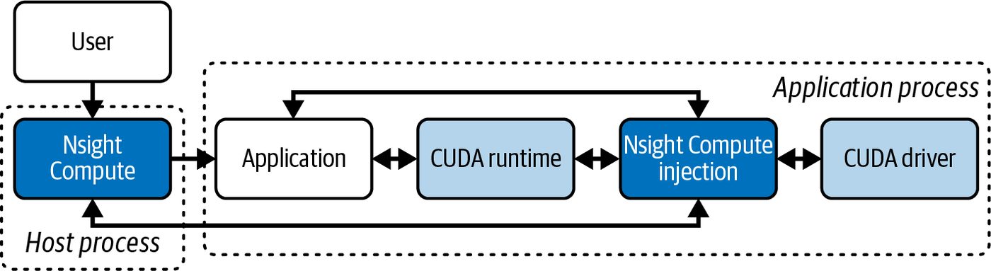
// Around kernel enqueues (compute stream) nvtxRangePushA("compute_stream"); my_kernel<<<grid, block, 0, compute_stream>>>(...); nvtxRangePop(); Here, we name the streams and wrap the enqueue sites in per-stream ranges so the Nsight timeline stays readable. It’s important to note that the NVTX ranges annotate the host-thread timeline. The GPU lanes show kernels/memcpys by stream. Naming the streams helps tie the host ranges to the right GPU lanes during analysis. Nsight Compute lets us profile individual kernels to pinpoint inefficiencies. We can use the Nsight Compute’s section-based profiling feature to focus on specific parts of the kernel, such as memory transactions. Another super useful tool that isn’t well known is Nsight Compute’s CUDA Program Counter (PC) Sampling feature. This samples program counters and identifies hot‐ spots without requiring full, heavyweight instrumentation, as shown in Figure 16-4.
Figure 16-4. Nsight Compute’s CUDA Program Counter (PC) sampling feature helps identify hotspots in a low-overhead manner (source: https://oreil.ly/DyKWR)
Profiling, Debugging, and Tuning Inference Performance | 711
Specifically, we can use this to profile live inference servers and pinpoint exactly which kernel instructions are taking the most time. And we can do this in a lowoverhead manner. Now that we’ve covered profiling with Nsight Systems and Nsight Compute, let’s discuss some common troubleshooting recipes for inference.
                         In production investigations on live services, prefer Program
                         Counter Sampling first to localize hotspots with minimal overhead.
                         Only switch to full tracing if the sample points to a specific kernel
                         or phase.
Inference Troubleshooting Recipes In production environments, it’s impractical to run heavy profilers continuously. As such, you need to rely on lightweight, metric-based monitoring such as GPU SM uti‐ lization, KV cache warnings, tail-latency percentiles, cache-hit rates, and OOM alerts to detect anomalies and guide targeted fixes. When a metric crosses a specific thresh‐ old, you can form a hypothesis about its root cause, such as a small batch size, insuffi‐ cient KV cache, routing hotspot, unbalanced sharding, memory overcommitment, etc. Then you apply a fix such as tuning batch sizes, raising memory-utilization limits (if possible), adjusting router thresholds, or enabling CPU offload. Once the fix is pushed, you should verify the impact and confirm that the metrics have settled below their thresholds. Table 16-1 shows some key metrics, symptoms, probable causes, and recommended fixes for common production issues.
Table 16-1. Common troubleshooting symptoms, causes, and recommended actions Metric/symptom Probable cause Recommended action SM utilization < 50% Small batches or lack of Increase batch size, enable fused kernels (FlashAttention or the fused kernels cuDNN-fused scaled_dot_product_attention (SDPA) backend in PyTorch), or add custom fused kernels (e.g., using Triton); then profile with nsys --trace=cuda. KV cache preemption Insufficient KV cache space Increase GPU memory utilization threshold, reduce max number of warnings (vLLM) batched tokens, consider PagedAttention for dynamic KV allocation. High tail latency (p95 Decode-node hotspot or Inspect router logs for routing patterns. Tune prefetch threshold. > 200 ms) head-of-line blocking Enable speculative decoding paths. Cache-hit rate < 60% Unbalanced shard Validate the prefix caching connector configuration (e.g., LMCache’s under load placement or missing prefix NIXL for vLLM and NVIDIA Dynamo’s NIXL connector), and increase cache prefix-cache TTL or replica count if needed. Unexpected OOM on Overcommitted GPU Lower per-instance GPU memory utilization, enable CPU/NVMe multitenant GPU memory offload, pin processes to CPU sockets to reduce cross-socket traffic. Irregular performance Mismatched clocks or Make sure all clocks are synchronized, and monitor for thermal and outliers thermal throttling power throttling.
712 | Chapter 16: Profiling, Debugging, and Tuning Inference at Scale
               Note: The numeric values in all metrics tables are illustrative to
               explain the concepts. For actual benchmark results on different
               GPU architectures, see the GitHub repository.
You may also find some of this information buried in logfiles. Cloud providers like AWS support regular expression (RegEx) filters on logfiles to extract numeric values from loglines and export them directly as metrics. AWS CloudWatch, for instance, supports this useful feature. There are example log lines in the next code block that are useful to monitor. Here is a sample vLLM log snippet that indicates KV cache preemption due to not enough KV cache space. As such, a KV recomputation was triggered, which uses more GPU compute resources and increases latency: WARNING 2025-05-03 14:22:07 scheduler.py:1057 Sequence group 0 is preempted by PreemptionMode.RECOMPUTE because not enough KV cache space. total_cumulative_preemption_cnt=1 Next is a sample NVIDIA Dynamo routing log. Here, the first line shows a 90% prefix-cache hit on the local decode worker, which kept the prefill running locally. The next line shows a local cache miss. The router then dispatches the prefill to the remote GPU-node-03 worker node: [Router] 2025-05-03T14:23:11Z INFO KVRouter: prefix-cache hit (90%) for model=DeepSeek-R1; routing to local vLLM worker [Router] 2025-05-03T14:23:12Z INFO KVRouter: cache miss; dispatching remote prefill to GPU-node-03
Full-Stack Inference Optimizations High-performance LLM inference demands coordinated optimizations across every layer of the stack. This includes everything from model architecture and kernel implementations to runtime engines, system orchestration, and deployment infra‐ structure. Model-level techniques like pruning, distillation, sparsity, MoE routing, efficient attention (e.g., FlashAttention), and quantization-aware training can reduce compute and memory requirements. At the kernel level, fused operations, custom attention engines (e.g., FlashInfer), Tensor Core utilization, block tiling, and asynchronous memory transfers will help maximize GPU throughput. Runtime strategies like dynamic batching, paged KV caches, CUDA Graphs, and overlap of computation and communication will keep GPUs saturated under variable loads. System orchestration layers can use prefill/decode disaggregation, intelligent routing, multitenancy isolation, and autoscaling (with warm spares) to balance latency and improve cost efficiency.
Profiling, Debugging, and Tuning Inference Performance | 713
                    Many production systems use Kubernetes-based orchestration to
                    run separate prefill versus decode deployments. They use ingress
                    controllers to route requests based on load or user priority. And
                    they keep warm standby GPU pods ready to spin up when traffic
                    spikes.
Finally, you should explore deployment patterns like geo-distributed edge serving, smart API gateway batching, CI/CD for model variants, and real-time profiling. This will provide peak reliability and adaptability in production. Table 16-2 describes some common optimization approaches for each layer in the stack.
Table 16-2. Common optimization approaches for each layer in the stack
Stack layer     Key techniques
Model           Pruning and knowledge distillation to shrink model size with minimal accuracy loss
                Sparsity (MoE) to skip computations
                Efficient attention (FlashAttention) to reduce memory footprint and intermediate buffers
                Quantization-aware training in FP16/BF16 or INT4/FP8 for robustness at low precision
Kernel          Fused operator kernels (e.g., Linear + GELU + LayerNorm) to reduce launch overhead and memory traffic
                Custom attention kernels (FlashInfer) for block-sparse KV- and JIT-compiled kernels
                Tensor Core and specialized instruction utilization (cp.async, TMA) for matrix ops
Runtime         Dynamic batching with latency controls as implemented in vLLM, SGLang, and NVIDIA Dynamo (e.g.,
                continuous batching) to consolidate requests
                Paged KV cache management to flexibly allocate memory and merge batches (vLLM’s PagedAttention)
                CUDA Graphs and buffer pooling to reduce per-inference overhead
                Use multiple CUDA streams (one stream for data transfer and another stream for compute) to overlap
                computation and communication. Use event-based synchronization—and only when needed.
System          Prefill–decode disaggregation for head-of-line blocking elimination
orchestration   Intelligent routing and cache affinity to balance load and cache hits
                Multitenancy isolation and per-user quotas to prevent noisy neighbors
                Autoscaling with warm spare instances to hide model load times and accept a slight cost increase for
                significantly better latency during traffic spikes
Deployment and Geo-distributed and edge deployment to reduce network RTT
infrastructure  Smart API gateways with request-level batching across server pools
                CI/CD pipelines for rolling out new quantized or kernel-optimized model variants in canary mode
                High-bandwidth interconnects (NVLink/NVSwitch and InfiniBand) and NUMA affinity between GPUs and
                CPUs for optimal memory access
QoS and scaling SLA-aware dynamic batching and tail-latency controls
                GPU isolation with MIG or stream priorities to enforce QoS
                Real-time profiling dashboards for TTFT, TPOT, utilization, and memory bandwidth utilization
                Dynamic parallelism switching (TP, PP, DP) based on workload characteristics
When optimizing, it’s important to consider cross-layer synergies. For instance, quantization (model) reduces memory footprint, enabling larger batch sizes (run‐ time) without OOM errors, which in turn allows orchestration components to merge more requests per GPU cycle.
714 | Chapter 16: Profiling, Debugging, and Tuning Inference at Scale
You should also have a profiling-driven focus. Continuous profiling should guide which layer to optimize next. For instance, after fusion and quantization, if the CPU becomes the bottleneck for preprocessing and postprocessing, invest in faster token‐ izers or offload some tasks to the GPU. There are always trade-offs to consider when applying optimizations. Techniques like layer-level CPU offload and advanced decoding methods add complexity. For exam‐ ple, speculative decoding adds a draft model, and Medusa adds multihead parallel decoding. These are typically reserved for extreme cases such as ultralong contexts or erratic latency variances. Lighter-weight methods, including sparsity, batching, and disaggregation, deliver the bulk of benefits in production. It’s recommended to adopt a full-stack optimization approach by aligning model architecture, kernel design, runtime behavior, system orchestration, and deployment strategies. This means keeping your software stack up to date, including CUDA, cuDNN, NCCL, etc. Newer versions often include the latest optimizations and bug fixes. A full-stack approach reduces the likelihood that each stack layer becomes a bottle‐ neck. This way, teams can systematically eliminate bottlenecks, achieve consistent low latency, and maximize hardware utilization for large-scale LLM inference.
Debugging Correctness Issues Monitoring can also help to catch anomalies caused by bugs. For instance, if memory usage keeps climbing over time, it may be caused by a memory leak in your CUDA kernel. It’s recommended to use Compute Sanitizer (compute-sanitizer) during testing to catch device memory errors, race conditions, and out-of-bounds accesses. An example is shown here: compute-sanitizer --tool memcheck your_binary If one GPU shows much lower utilization than others, it might have dropped out of the NCCL communication group due to a silent NCCL failure or uncaught error. You can check for NCCL error codes in logs by looking for WARN NCCL_COMM_FAILURE. It provides very verbose error logs.
               Enable NCCL debugging by setting the environment variable,
               NCCL_DEBUG=WARN. This will help surface errors that would other‐
               wise be silent. Be warned, however, that NCCL logs are very
               verbose!
Use the NCCL test suite to debug all-reduce and all-to-all performance and correct‐ ness issues. You can also use ncclCommGetAsyncError with ncclCommAbort to detect and handle asynchronous communication errors. Consider enabling NCCL’s IB GID
Profiling, Debugging, and Tuning Inference Performance | 715
tracing and using NVSwitch system telemetry to detect issues at the interconnect level as well. You should set up alerts in Prometheus’s alert manager to detect unusual patterns like “GPU utilization < 10% for at least 60 seconds,” “memory usage above W% thresh‐ old,” “NVLink error rate > X,” “PCIe replays above Y threshold,” “temperature above Z degrees,” etc. In practice, you might configure Prometheus Alertmanager rules, as shown in Table 16-3. This way, you can proactively investigate issues.
Table 16-3. Example set of common Prometheus alerts for GPU-based systems Metric Condition Severity Notes GPU utilization < 10% for > 60 s Idle Underutilization GPU utilization > 90% Bottleneck Possible saturation Memory usage > 80% Warning Approaching OOM Memory usage > 95% Critical High risk of out-of-memory errors Temperature > 85 °C Warning Approaching thermal throttling Temperature > 95 °C Critical Risk of shutdown or hardware damage NVLink replay/recovery errors ≥1 Critical Indicates link retry or recovery NVLink CRC errors > 100 errors/sec Critical High CRC failure rate on link PCIe replay errors ≥1 Critical Packet retries on PCIe bus Uncorrectable ECC errors ≥1 Critical Data corruption requiring reset
You also want to set up hardware error counters and alerts as well. For example, if ECC errors or NVLink retries are reported, alert immediately, as these can quickly degrade performance or cause drop-outs. Dropouts happen when a GPU—or its interconnect—silently disconnects. For instance, an NVLink might drop—or the GPU might “drop off the bus” after a fatal error.
                     Use DCGM for per-link NVLink throughput and totals including
                     DCGM_FI_DEV_NVLINK_TX_BANDWIDTH_L*,
                     DCGM_FI_DEV_NVLINK_RX_BANDWIDTH_L*, and *_TOTAL. Fall back to
                     nvidia-smi nvlink, Nsight Systems/Compute, or NVSwitch coun‐
                     ters if needed.
Consider a NCCL failure case. You might get an alert that shows one node’s GPUs are near 0% utilization, while others are at 90%. You can start debugging the issue by checking the node logs and finding which node is generating the NCCL errors. This type of active monitoring and alerting lets you catch these issues more quickly, find the failed node, and start restoring it back to normal. In this case, you might
716 | Chapter 16: Profiling, Debugging, and Tuning Inference at Scale
want to reinitialize the NCCL communicators or perform a full node reboot (just make sure the node rejoins the NCCL group after restart/reboot). You could catch these issues even quicker by incrementing a “NCCL Error” counter for NCCL errors. In addition, your inference server can log the NCCL errors, which will automatically be scraped by Fluentd or AWS CloudWatch and convert them into counters. Then you can overlay the error counter chart on top of the per-node GPU utilization chart in Grafana. This will correlate the NCCL errors with a drop in GPU utilization so that you can identify and remediate the failed node much quicker.
               Application-level counters are extremely useful in production—
               especially when combined with system metrics.
And optimizations should not be considered successful until they are verified with actual metrics that demonstrate increased throughput, reduced latency, improved uti‐ lization, etc. A rigorous measurement-driven approach to system performance tuning is essential given the complexity of modern AI inference systems. In short, you should combine application-level counters, automatically scraped log counters from Fluentd or AWS CloudWatch, and low-level system metrics. This type of full-stack telemetry provides the visibility needed to operate—and optimize—a multinode LLM inference system running at peak performance on production work‐ loads. You should treat metrics, counters, and logs as the ground truth of your sys‐ tem’s behavior.
               Our intuitions and gut feelings can often lead us down the wrong
               debugging path. But metrics don’t lie. Instrument your code prop‐
               erly upfront—and trust the metrics when things go wrong.
Dynamic Batching, Scheduling, and Routing Even after the model has been partitioned and parallelized optimally across the clus‐ ter, there are still more opportunities for application-level optimizations in a multi‐ node inference cluster deployment. In this section, we focus on techniques to maximize GPU utilization, minimize latency, and boost throughput by dynamically batching requests and using optimized scheduling and routing strategies.
Dynamic Batching, Scheduling, and Routing | 717
Dynamic Batching One of the most powerful performance techniques in an inference serving system is batching. By combining multiple incoming inputs into a single batch for the model to process together, batching improves throughput by amortizing fixed costs—like ker‐ nel launches and memory loads—over multiple inputs. It does this at the expense of individual-request latency, however. Some individual requests may need to wait for a period of time (e.g., 2 ms) to join a batch and be processed. Dynamic batching is a specialization of request batching that assembles batches of incoming inference requests of dynamic sizes on the fly. It can be configured to buffer requests for a period of time or until a given batch size is reached. All modern LLM inference engines support dynamic batching, including vLLM, SGLang, and NVIDIA Dynamo. Dynamic batching is in contrast to static batching, which locks in a fixed batch size (or pads all sequences to the longest one) and then waits for every request in that batch to finish before returning results. This can incur unbounded queuing delay for early arrivals—and leave GPU cycles wasted on padding. With dynamic batching, the system accumulates incoming requests and dispatches “whatever has arrived” once either a target batch size is met or a short timeout (e.g., 2 ms) elapses. This bounds maximum latency to the timeout value that you specify. With its on-the-fly sizing, dynamic batching lets you amortize kernel-launch over‐ heads across multiple sequences—while avoiding the worst‐case delays of static batching. This improves both GPU utilization and predictable latency under variable load. Figure 16-5 shows the difference between static batching and dynamic batching.
Figure 16-5. Difference between static and dynamic batching
Dynamic batching lets the system automatically grow or shrink batch sizes based on actual request-arrival patterns and latency targets (e.g., max delay). The key is to batch intelligently in a way that increases overall throughput while maintaining latency within acceptable bounds. Modern inference engines implement microbatch‐ ing, which accumulates requests for only a few milliseconds before dispatching the
718 | Chapter 16: Profiling, Debugging, and Tuning Inference at Scale
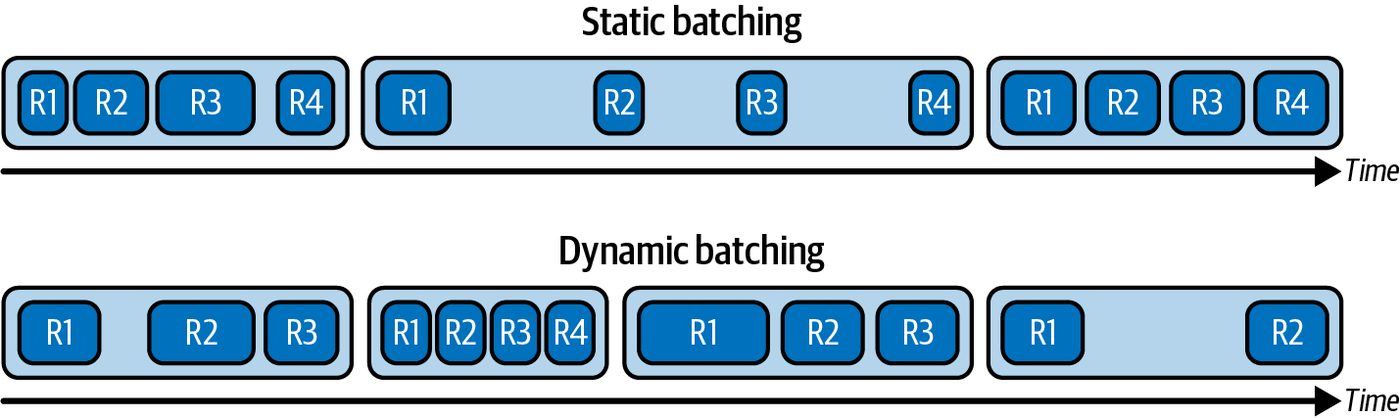
batch to the GPU. Typically, a delay of 2–10 ms is used, but this should be tuned to meet latency SLOs. For example, you can configure a batch delay of 2 ms to determine how long the server waits for additional requests before dispatching a batch. If three requests arrive within that interval, the batcher immediately groups and sends them to the GPU. Any further requests that arrive after the 2 ms timer expires will be collected into the next batch. This timeout-driven trigger bounds per-request queuing latency (never exceeding 2 ms) while improving throughput by grouping multiple sequences together. These microbatches reduce the delay added and allow the GPU to work on multiple requests at once—instead of one at a time. Large LLM models are memorybandwidth-bound at small batch sizes, so increasing the batch size will improve arith‐ metic intensity—and overall hardware utilization. In practice, LLM serving systems pick a balanced batch size that gives good through‐ put without incurring much latency. Under high load, dynamic batching can improve both throughput and latency because it prevents the GPU from sitting idle between requests. In fact, if the arrival rate of requests is high, batching can reduce overall queue wait times since more work is processed in the same amount of time. This ben‐ efits end-to-end latency and tail latency for high-load traffic patterns. Dynamic batching will, at low RPS (requests per second), add a small delay as it waits for other requests to join the batch. This will slightly increase latency at low RPS. However, at moderate to high RPS, the delay is amortized and becomes negligible compared to the queuing delay that would occur if we ran everything one by one. As such, batching lowers overall latency, including tail latency.
                You should validate the improvement by plotting latency percen‐
                tiles against load using tools like Grafana. With batching, you’ll
                often see overall p50 latency stay flat—or even drop—as through‐
                put increases. This will happen up until an inflection point. Make
                note of this inflection point and stay under this value.
It is important to configure batching with respect to latency SLOs. For instance, if you promise a p99 latency of 2 seconds for a request of a certain length, you can’t afford to delay one request by 500 ms waiting in a batch queue. By default, your dynamic batch delay should be initially set well below the p99 latency requirement (on the order of 1–2 ms) to avoid excessive batch delays. Using an adaptive batching delay, the batch delay value can dynamically drop to near 0 ms at low RPS and increase higher to 5–10 ms at peak load when needed. This adaptive approach is used by vLLM and others to maintain SLO compliance across different traffic patterns.
Dynamic Batching, Scheduling, and Routing | 719
Batching primarily benefits high-traffic scenarios. If traffic is low, the system will just run single requests, and the latency will be very low. At high load, however, the system can apply aggressive batching to achieve high throughput and will provide better overall latency since it avoids queue buildup and amortizes the latency across many requests.
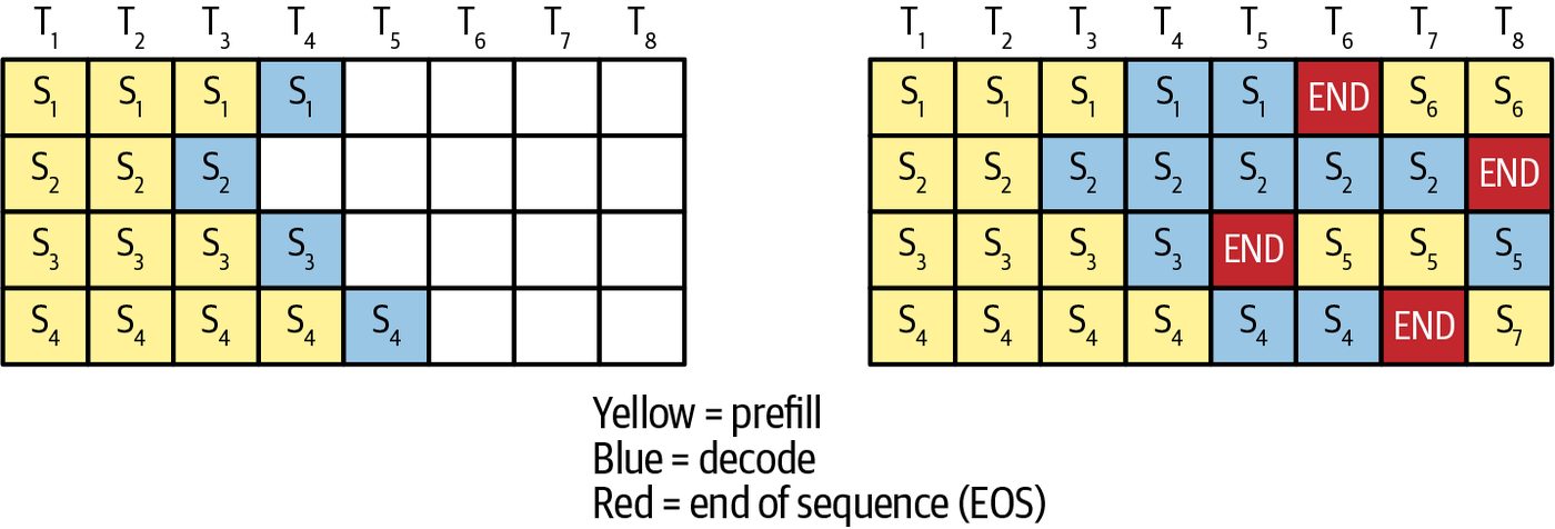
Continuous Batching Continuous batching, also known as in-flight batching or iteration-level scheduling, maintains high GPU utilization by refilling batches on every token-generation itera‐ tion rather than waiting for complete sequences to finish. It evicts completed requests and immediately pulls in new ones based entirely on GPU readiness. This technique is particularly important for low-latency use cases such as chat assistants. In contrast to timeout-driven approaches like dynamic batching, the event-driven continuous batching strategy eliminates idle compute slots and the padding overhead of these other approaches. By never relying on a fixed “max-delay” timer, continuous batching allows new requests to join an ongoing batch mid-generation—and without blocking on the longest sequence, as shown in Figure 16-6.
Figure 16-6. Continuous batching allows new sequences (requests) to join a batch mid-generation
Here, continuous batching minimizes wasted slots in the inference compute pipeline. It eliminates the idle time caused by waiting for the longest response to finish for each batch. Instead of waiting for all sequences in a batch to finish (which is inefficient due to variable output lengths and leads to GPU underutilization), continuous batching replaces completed sequences with new ones at each iteration. This approach allows new requests to fill GPU slots immediately—resulting in higher throughput, reduced latency, and more efficient GPU utilization. Batching 4–8 requests can often double or triple the throughput over 1–2 request batches on large models. This is because the GPU’s math units and memory pipelines are better utilized. And the additional latency per request is on the order of only a few
720 | Chapter 16: Profiling, Debugging, and Tuning Inference at Scale
milliseconds—making this strategy ideal for low-latency use cases. Table 16-4 summarizes the different batching strategies discussed so far, including a naive static batching strategy.
Table 16-4. Comparing static, dynamic, and continuous batching
Aspect              Static batching            Dynamic batching                              Continuous batching
Trigger             Fixed batch size or        Batch-size target or timeout                  Token-generation
                    sequence length                                                          completion event
Latency bound       Unbounded; wait for full   Bounded by max_batch_delay_ms                 Minimal; evicts and refills
                    batch                                                                    mid-batch
Padding overhead High overhead: pad to         Moderate overhead: pad within each batch      Low: slots refilled without
                    longest sequence                                                         waiting for padding
GPU idle mitigation Poor: especially under     Better: but can cause idle GPU if the timer   Excellent: keeps GPU
                    variable-sized loads       fires on a small batch                        saturated at every iteration
Implementation      Simple                     Moderate: requires timers and queue           Complex: requires per-token
                                               management                                    coordination and state
                                                                                             tracking
Continuous Scheduling Another dimension of request scheduling involves concurrent model execution. The vLLM community calls this continuous scheduling. The idea is that if the model is small—or if the batch size is limited by latency targets—a single model instance might not fully saturate the GPUs. Continuous scheduling treats the GPU like an OS scheduler treats a CPU. It launches independent small kernels on separate CUDA streams. This lets the hardware warp scheduler interleave warps across tasks without explicit context switching. For example, if our inference engine is not fully saturating the GPUs, it can run mul‐ tiple model inference streams concurrently on the same GPU. This way, while one instance is waiting on a data transfer or a non-GPU operation, another instance can execute. Specifically, during the decode phase, generating one token at a time can often leave the GPU underutilized—especially if performed on a single sequence of text. This is because the workload is relatively small and requires a large amount of memory movement relative to the amount of compute. To address this inefficiency, the inference engine can interleave multiple decode tasks from across different user requests. For example, if 10 users are decoding different sequences at the same time, you can’t simply batch them into one large matrix multi‐ ply. This is because each sequence may be a different length. This would prevent the GPU from performing efficient matrix operations without requiring a large amount of padding.
Dynamic Batching, Scheduling, and Routing | 721
Instead, the continuous scheduler can launch 10 small decode kernels for each sequence’s next token in rapid succession on separate CUDA streams. This allows true concurrency across sequences by utilizing the GPU’s fine-grained warp schedu‐ ler. As such, the kernels interleave execution across SMs. This prevents idle cycles by approximating a round-robin processing pattern. By enqueuing each decode task on its own stream, the GPU can overlap memory transfers and computation across sequences. This reduces per-token latency and improves overall throughput. The GPU switches between the kernels at the warp level. And when one decode ker‐ nel stalls due to inefficient control flow on the CPU or a network I/O wait, other active kernels can immediately proceed. This keeps the GPUs fully utilized. Continuous scheduling achieves high utilization even at token-level granularity by maintaining a queue of ready-to-run token tasks. The end result is similar to batch‐ ing. The GPU is always working on token generation, but it doesn’t require combin‐ ing them into one giant matrix multiply. It just means that we don’t let the GPU sit idle between token computations. This type of token-level granularity scheduling is essential to maximizing throughput across millions of users. At fixed intervals or whenever the GPU frees up, a continuous scheduler gathers all pending next-token requests into a configurable-sized batch and then dispatches the batch as a single GPU call. This helps balance throughput and latency.
                     If you are designing a custom scheduler, consider the hybrid
                     approach: use a short timer and a maximum batch size for token
                     scheduling.
State-of-the-art systems like vLLM and SGLang merge dynamic batching with con‐ tinuous scheduling. Their custom continuous scheduler is built around the idea of squeezing out “bubbles” of GPU time. vLLM’s PagedAttention is a specific example of this hybrid approach. PagedAttention breaks the attention key-value (KV) cache into slices, or pages, and dynamically groups the page-specific compute across active sequences. This sustains near-100% GPU utilization under heavy load by interleaving large prefill GEMMs with rapid, small decode kernels. vLLM efficiently uses block-level KV cache structures to track each request’s state separately. This fine-grained bookkeeping provides fast streaming responses and optimal hardware utilization by continuously packing and multiplexing workloads in real time.
722 | Chapter 16: Profiling, Debugging, and Tuning Inference at Scale
Another example is SGLang’s RadixAttention, which uses tree-based KV cache grouping. This achieves similar near-100% GPU utilization and introduces lazy evic‐ tion for unused cache pages. We’ll cover vLLM’s PagedAttention and SGLang’s RadixAttention in more detail in a bit. Both approaches are open source, so you can review their scheduling implementations directly in code.
Stall-Free Scheduling (Chunked Prefill) When prompts are extremely long, you can split them into chunks and interleave the prefill and decode work. This is called stall-free scheduling or chunked prefill. Consider a 20K token prompt. By splitting the prompt into 5K token chunks, you reduce the maximum stall per iteration and bound the per-iteration work to a fixed number of tokens. This provides predictable per-iteration latency. The cost of chunked prefill for different chunk sizes is shown in Table 16-5.
Table 16-5. Cost for a 20 K token prompt using chunked prefill of different chunk sizes Chunk size Number of chunks Attention ops per chunk Total MLP tokens 20K 1 20K × (20K + 1) ÷ 2 = 200M 1 × 20K = 20K 10K 2 50M + 150M = 200M 2 × 10K = 20K 5K 4 12.5M + 37.5M + 62.5M + 87.5M = 200M 4 × 5K = 20K
Here, the per-chunk attention cost grows with the full context due to KV caching. Each new chunk computes attention for its own tokens against all prior tokens from previous chunks. In self-attention, the number of QK dot products for a sequence of length N is trian‐ gular, approximately N(N + 1) ÷ 2. This is the number of Q × K dot product opera‐ tions per layer per head. This cost is quadratic in N (O(N2). So for N = 20,000, this is about 200 million operations. Chunking does not reduce this total. Chunking only changes when work becomes available to the decoder. The benefit of chunked prefill is latency smoothing and improved overlap, not fewer total attention dot-product operations.
                   Prefill self-attention performs N(N + 1) ÷ 2 Q × K dot products per
                   layer per head. This cost is quadratic in N, O(N2). Note that chunk‐
                   ing and pipelined prefill change only overlap and latency; they do
                   not change the total amount of attention work. The only ways to
                   reduce the total attention cost are to reduce the effective context or
                   to use local or sparse attention. For example, you can reduce the
                   cost to O(NW) with a fixed attention window W.
In short, the chunked prefill technique schedules prompt prefill processing and token generation in a tightly interleaved way. It unifies the high efficiency of large-batch
Dynamic Batching, Scheduling, and Routing | 723
prefill compute with the responsiveness of streaming decode. This can lower tail latency while maintaining high throughput on many workloads.
Latency-Aware Scheduling and Dynamic Routing Latency-aware scheduling can analyze incoming requests, create dynamic batches, and route the batches to minimize latency. Consider six prompts arriving into a twoGPU inference system at the same time. The prompt lengths are 6K, 2K, 6K, 2K, 2K, and 2K in that order. Let’s compare a naive first-in-first-out (FIFO) scheduler with a latency-aware scheduler. First, the FIFO scheduler creates two batches based on arrival order. Batch 1 is [6K, 2K, 6K] and is sent to GPU 1. Batch 2 is [2K, 2K, 2K] and is sent to GPU 2. The results are summarized in Table 16-6.
Table 16-6. FIFO versus latency-aware scheduling for a sequence of incoming prompts of length [6K, 2K, 6K, 2K, 2K, 2K] GPU Prompt batch Self-attention QK ops T(N) = N(N + 1) ÷ 2 Tokens N GPU 1 6K, 2K, 6K T(6K) + T(2K) + T(6K) = 18,003,000 + 2,001,000 + 18,003,000 = 38,007,000 14K GPU 2 2K, 2K, 2K 3 × T(2K) = 3 × 2,001,000 = 6,003,000 6K
Here you see that the FIFO strategy sends the first three prompts [6K, 2K, 6K] to GPU 1 for approximately 38,007,000 self-attention Q × K dot products and 14,000 tokens of MLP, while GPU 2 sees approximately 6,003,000 self-attention Q × K com‐ putations and 6,000 tokens of MLP. The critical path is determined by GPU 1 at approximately 38,007,000 self-attention Q × K dot products. In contrast, the latency-aware scheduler analyzes the expected latency of the six requests and rearranges them into two batches of [2K, 2K, 6K]. In this strategy, the self-attention cost per GPU is 22,005,000 dot products with 10,000 tokens of MLP, as shown in Table 16-7.
Table 16-7. Latency-aware scheduling for prompts of length [6K, 2K, 6K, 2K, 2K, 2K] in that order GPU Prompt batch Self-attention QK ops T(N) = N(N + 1) ÷ 2 Tokens N GPU 1 2K, 2K, 6K T(2K) + T(2K) + T(6K) = 2,001,000 + 2,001,000 + 18,003,000 = 22,005,000 10K GPU 2 2K, 2K, 6K T(2K) + T(2K) + T(6K) = 2,001,000 + 2,001,000 + 18,003,000 = 22,005,000 10K
This reduces the critical path self-attention by about 42% from 38,007,000 to 22,005,000. As such, the latency-aware scheduler can significantly reduce TTFT. Because the latency-aware scheduler is aware of prompt lengths, the triangular N(N + 1) ÷ 2 cost in self-attention, and the O(N) cost in MLP, it can balance compute weight and minimize overall latency. For instance, in this example, the latency-aware
724 | Chapter 16: Profiling, Debugging, and Tuning Inference at Scale
scheduler moves the 2K token requests earlier. This allows these lighter requests to finish prefill sooner and begin decode without waiting for the heavier 6K token prefill to complete.
               These counts assume a variable-length fused attention kernel that
               computes only over valid tokens—for example, FlashAttention or
               PyTorch scaled dot product attention (SDPA) with the cuDNN
               backend. If your kernel pads to the maximum sequence length in a
               batch, the attention arithmetic cost approaches the batch size mul‐
               tiplied by T tokens of the longest sequence in that batch. In this
               case, the difference between FIFO and latency-aware strategies will
               shrink.
In short, a naive FIFO scheduler can overload one of the GPUs if the arrival order is not globally ideal within the batch. A latency-aware scheduler can analyze incoming requests and rearrange them into more balanced batches to minimize latency.
               Some inference serving frameworks have incorporated reinforce‐
               ment learning to adjust scheduling policies online. This builds on
               the latency-aware strategies described here by automatically tuning
               for changing traffic patterns.
Systems-Level Optimizations Systems-level optimization techniques include overlapping communication with computation, maximizing GPU utilization, managing power and thermal concerns, handling errors, and optimizing memory access. Overall, we’re making sure that our GPU hardware is doing useful work, or goodput, nearly 100% of the time. We also discuss the trade-offs between throughput and latency and how to find a balance appropriate for production SLOs.
Overlapping Communication and Computation As we’ve seen repeatedly throughout this book, overlapping communication with computation is critical for inference performance with large models distributed across many GPUs. The massively high bandwidth of systems like the GB200/GB300 NVL72 (up to ~130 TB/s of aggregate GPU-to-GPU NVLink bandwidth within a rack) means that overlap is even more effective because data transfers are fast enough that computation is less likely to be starved. However, even with the NVL72, it’s criti‐ cal to use multiple CUDA streams and nonblocking collectives. This will allow you to perform communication-compute overlap to hide latency and keep all 72 GPUs busy—even at these speeds.
Systems-Level Optimizations | 725
                     In practice, you want to enable NCCL’s GPUDirect RDMA
                     support—and use NCCL’s group calls to overlap multiple small all-
                     reduce operations. Also, consider using SHARP (available on
                     InfiniBand with suitable switches) to offload reduction operations to
                     the network fabric. This optimization can improve throughput on
                     some fabrics and topologies. In some tests, it has shown roughly
                     10%–20% throughput improvements for large all-to-all
                     communications.
Consider an inference step that requires transferring data between GPUs (e.g., all-toall for MoE)—or even just sending the prompt data from CPU to GPU and the response from the GPU to the CPU to return to the end user. In all of these scenarios, we want to perform these transfers asynchronously while the GPU is doing other work, whenever possible. One basic example is using separate CUDA streams to overlap compute and data transfer. For example, launch cudaMemcpyAsync on a dedicated transfer stream (with pinned host memory) while compute kernels run on the default stream.
                     Remember to use page-locked host buffers for transfers over PCIe
                     or NICs. This way, the CUDA driver can DMA directly and overlap
                     with compute.
You would then synchronize with a CUDA event only when the data is needed. This prevents the GPU from idling on I/O. This way, data transfers will use nonblocking CUDA calls (e.g., pinned memory) and CUDA streams so that the GPU doesn’t stall waiting on these operations. On modern GPUs with full duplex NVLink bandwidth, such overlap can largely hide communication latency. However, you should verify this with profiling on your specific workload. Data transfers in this context can include sending new prompt embeddings from the CPU to the GPU—or moving the last token’s logits from the GPU to the CPU. For instance, right after a GPU computes the logits for a batch of new tokens, we can kick off an asynchronous copy of those logits to the CPU for postprocessing (e.g., sam‐ pling)—or for sending back to the client as a streaming response—and immediately launch the next compute kernel for another batch of tokens that are still on the GPU. In multinode scenarios, a communication collective like all-to-all can overlap by dividing work into chunks. A technique used in some MoE runtimes is to split the batch of tokens into two halves, and, while the first half ’s tokens are being processed by experts, it can start sending the second half ’s tokens.
726 | Chapter 16: Profiling, Debugging, and Tuning Inference at Scale
By the time the experts finish with the first half, the second half ’s data has arrived at the destination GPUs—and they can proceed without waiting. This requires careful scheduling of the NCCL calls relative to compute kernels. For example, you can implement this overlap using CUDA events to signal when half the batch is done. At this point, you can launch the NCCL all-to-all for that portion of the data—while the next portion finishes computing. You can use CUDA Graphs to capture these asynchronous patterns and reduce launch overhead. The result is improved GPU utilization because the GPUs spend less time sitting idle waiting for communications. Another area of overlap is between the CPU and GPU. For instance, while the GPU is busy generating the next token, the CPU can concurrently prepare the next input or perform result handling for previously generated tokens. A highly optimized infer‐ ence engine will overlap any CPU-side preprocessing (e.g., input-text tokenization) in parallel with GPU computations from other requests. For example, the engine can prepare the next batch while overlapping with GPU computations of the current batch. This sounds obvious, but it requires a multithreaded architecture such that one thread handles networking and queuing, while another thread launches GPU opera‐ tions. And yet another thread might handle response postprocessing, etc. The Python or C++ inference loop should never block the GPU from starting new work due to waiting on an operation that could otherwise be done concurrently. In pipeline parallel scenarios, the system should overlap communications (between pipeline stages) with computations inside of each stage. For instance, GPU 0, after finishing its part for token t, can start sending activations to GPU 1 at the same time as it begins processing token t+1 for another sequence. Modern interconnects and frameworks allow compute kernels and data transfers to overlap as long as they use different resources. You should use multiple CUDA streams in an inference pipeline such that each pipeline stage has an independent stream. This way, the sending/receiving of activations can happen in parallel with other streams that are performing computations for different microbatches. The effect is that pipeline bubbles are reduced. On the networking side, technologies like NVIDIA GPUDirect RDMA allow network adapters like InfiniBand NICs to read and write GPU memory directly without involving the CPU—and without staging through host memory. By utilizing GPU‐ Direct for cross-node transfers of KV cache or expert activations, the inference engine reduces latency and CPU overhead. GPUDirect RDMA removes staging through host memory and allows the NIC DMA engines to access GPU memory directly. The CPU posts work requests, but the data path bypasses the CPU. This frees CPU cores for other tasks.
Systems-Level Optimizations | 727
Consider a practical example using InfiniBand for all-to-all communication in an MoE layer across two NVL72 racks. If you do this synchronously by first performing the all-to-all and then computing, the GPU utilization can remain low without over‐ lap. By overlapping batches of the all-to-all communication with compute, however, you can significantly increase GPU utilization. Overlapping all-to-all communication in an MoE layer involves splitting the token batch in half and beginning the second half ’s exchange while the first half ’s experts are still computing. This hides communication latency by interleaving it with compute. Essentially, each GPU begins computing its local experts’ outputs for the tokens it already has—while simultaneously receiving the remaining tokens from the other node. By the time it finishes the first batch, the second batch has arrived and can be computed immediately. This kind of optimization is fairly low level and involves CUDA event synchroniza‐ tion between NCCL groups and CUDA streams, but it produces worthwhile through‐ put improvements and smoother latencies. In practice, you first launch the NCCL allto-all as part of a NCCL group without waiting for completion. Then you immediately launch the next compute kernel. Make sure to check for completion using CUDA events. We can also overlap I/O with compute for streaming outputs. For instance, as soon as a few tokens are generated, we send them over the socket to the end user—while the model is already working on the next tokens. This hides the network latency (e.g., sending the response back to the end user) behind computation (e.g., subsequent tokens). As such, the end user sees a steady stream without pauses. This pattern of nonblocking streaming to clients is adopted in all modern LLM infer‐ ence engines. They use separate threads for sending token updates to clients using SSE/WebSockets.
                     If you are implementing streaming outputs yourself, make sure to
                     use thread-safe queues or locks to hand off generated tokens to the
                     networking thread. You don’t want to introduce synchronization
                     issues in this handoff. These can be very difficult to identify and
                     debug.
If we didn’t overlap, we would generate a small number of tokens and then have the GPUs sit idle while we send the tokens back to the end user. Instead, our network send is handled by an async thread that takes the output from the response buffer and streams it back to the user. This allows the main inference thread (e.g., CUDA stream) to immediately continue generating more tokens. This effectively pipelines token generation (compute) with output transmission (I/O).
728 | Chapter 16: Profiling, Debugging, and Tuning Inference at Scale
In short, overlapping communication and computation requires thinking in terms of pipelines and using asynchronous operations whenever possible. Modern GPUs and networking hardware provide the primitives to implement this, including CUDA streams, nonblocking collectives, and RDMA. CUDA device-side primitives such as cuda::memcpy_async used with cuda::barrier (from the CUDA pipeline header) help overlap global to shared memory movement with compute inside a kernel. (Note: Host-to-device and device-to-host transfers still require explicit CUDA streams and pinned host memory to overlap with compute.) Efficient LLM inference systems take full advantage of these features. In short, always overlap communication with computation whenever possible. Other‐ wise, scaling to many GPUs—even with NVLink/NVSwitch—will fall short of peak hardware performance. These optimizations are mostly invisible to the end user since there’s no change in model outputs. However, these are essential to squeeze out every bit of performance from the inference cluster and keep users coming back to your application.
Maximizing GPU Utilization and Throughput Versus Latency Trade-Offs The ultimate goal of performance tuning is to keep GPUs as busy as possible doing useful work, such as matrix multiplies—while minimizing any idle and underutilized GPU resources. Many of the techniques described previously, including batching, parallelism, and overlap, are designed to achieve near-100% GPU utilization. GPU utilization percentage—and specifically useful utilization, or goodput—is an important performance metric to monitor continuously. And while you want to push for 100% useful utilization, you need to make sure you are not violating your SLOs, such as latency. At some point, you may reach a point of diminishing returns. Consider an inference server that is currently showing 60% GPU utilization with a naive implementation. Investigating, you find that the decode stage is a bottleneck because it’s waiting for a single thread to handle all sequences sequentially. Let’s intro‐ duce concurrent decoding using multiple streams. By interleaving decodes, as described earlier, we raise GPU utilization to 95% and double the throughput. This confirms that concurrent decoding is working. We can try to reach 100% by putting more requests into a massive batch, but this will slow down individual queries. It’s often helpful to plot a throughput-versus-latency curve by testing various batch sizes. In this chart, there’s usually a sharp “knee” where throughput gains start costing too much latency. To find the sweet spot in the throughput-latency curve, first turn on full concurrency and overlap as much as possible so you know the hardware can stay busy. Then grad‐ ually increase the batch size until you hit maximum resource utilization. At this point,
Systems-Level Optimizations | 729
measure single-query latency and scale back just enough (e.g., from 16 to 8) to meet your response-time targets. It’s recommended to monitor your p95 and p99 tail latencies along with p50 median latency. This is because small jitters and uneven batch fills can produce long-tail out‐ liers noticeable at p95/p99. In a large cluster serving many requests, even a 0.1% out‐ lier can occur frequently. Thus, p99—or even p99.9—might be more important than p50 for measuring user experience. In addition, long-tail latency often forces over‐ provisioning to meet aggressive SLOs. As such, reducing tail latency has direct cost benefits.
                     A good rule of thumb is to cap your batch size slightly below the
                     one that gives peak throughput. Teams typically target 90% of max‐
                     imum peak throughput, called the headroom buffer. This is because
                     running at full speed can cause unpredictable latency spikes. For
                     instance, if increasing the batch size to 16 requests starts to add a
                     small amount of latency to a few requests, you should reduce the
                     batch limit to 8. This will provide more consistent latency and
                     reduce throughput only slightly.
Some inference systems can dynamically adjust the batch size on the fly based on these metrics. We’ll cover this technique—and many more adaptive inference strategies—in Chapters 17–19. It’s important to remember that running GPUs at a constant 100% can cause throt‐ tling by hitting power and thermal limits. Sometimes running at 90% with efficient kernels can outperform 100% with throttling. Next, let’s discuss GPU power and ther‐ mal constraints—characteristics that CPU-based application developers and systems engineers often don’t consider.
Power and Thermal Constraints Another dimension to consider is power and thermal constraints. Continuously run‐ ning GPUs at 100% will cause thermal throttling if cooling is insufficient. Modern GPU systems are liquid-cooled to reduce thermal throttling and sustain performance. If you’re running older, air-cooled systems, watch out for downclocks. You can monitor downclocks with nvidia-smi or DCGM when GPU utilization is high. Specifically, DCGM exposes XID throttling reasons through DCGM_FI_ DEV_CLOCK_THROTTLE_REASONS. And nvidia-smi will show a “Pwr Throttle” flag when a GPU is being power-throttled. You may also hit power limits on the board—especially with boost clocks. Modern GPUs draw significantly more power under boost, so you should monitor if GPUs downclock due to hitting a power limit. If this happens, you will experience
730 | Chapter 16: Profiling, Debugging, and Tuning Inference at Scale
less-than-ideal GPU performance. Always monitor the DCGM_FI_DEV_POWER_USAGE metric from DCGM and alert anytime this exceeds the normal range.
                If your GPUs consistently hit power limits, consider enabling
                Dynamic Boost mode—or underclocking slightly—to avoid ther‐
                mal throttling that can spike latency.
To work around these constraints in software, you can slightly ease off utilization by adding a tiny interbatch delay. You can also limit concurrency. Modern GPUs also support clock capping. So rather than adding delay, you could cap the GPU clocks marginally using nvidia-smi -lgc or similar to prevent hitting thermal limits. This will only slightly reduce throughput—and provide more consistent performance. From a hardware perspective, you can try to improve cooling or raise the power limit if cooling is already adequate. To increase the power cap, use nvidia-smi -pl or tune your GPU boost settings. These are all reminders that pushing real-world systems to their limits can cause unexpected side effects that greatly impact performance. It’s recommended to include a “boost-off ” flag in your inference engine to apply the software workarounds on the fly when the system detects performance degradation due to throttling caused by power or thermal constraints. This will run your system in a slightly underutilized and cooler state until full stability and performance are restored.
Error Handling While not typically associated with performance, it’s important to handle errors effi‐ ciently. A fully utilized inference system has less headroom to handle excessive error spikes—especially since error handling is likely not the most optimal code path in your system. In failure scenarios, failing fast is the key since, if a request will error, it’s best to return the error immediately rather than waste GPU time with a slow failure. Be sure to implement proper exceptions and timeouts around inference calls to catch hangs or crashes. Additionally, it’s recommended to implement backpressure. This means that if errors spike, you can start rejecting new requests—or reduce batch sizes—to give the system some headroom to recover. At scale, it’s recommended to build in some headroom, adding some extra replicas that sit mostly idle. These can act as a buffer for spikes in errors or other unexpected situations. While autoscaling is likely the first option you think of to reduce cost, just remember that autoscaling takes time to provision the new resources.
Systems-Level Optimizations | 731
While idle capacity costs money, the cost of lost customers or SLA violations is often higher. At least 10%–15% of buffer capacity is recommended during steady state. For more critical services that cannot incur downtime, it’s recommended to provision 100% buffer capacity—or a full cluster replica. There is simply no substitute for prewarmed, idle nodes that can handle the extra load immediately on demand. The cost of losing end users is likely higher than the cost of keeping a few replicas idle and ready to handle any additional, unexpected load.
Memory Optimizing resource utilization extends to memory as well. While GPU memory and memory bandwidth are growing somewhat incrementally, model sizes and context lengths are growing exponentially. As such, memory remains a precious resource to optimize—and will remain precious in the near future. As such, you want to utilize GPU memory and memory bandwidth effectively. Mem‐ ory is typically filled by the model weights and KV cache. During inference, it’s best to keep the model weights in GPU HBM at all times. If you page memory in and out of CPU DRAM or NVMe storage, you will incur extra page faults and transfer latency. This additional transfer latency is true even for modern CPU-GPU superchips like Grace Blackwell and Vera Rubin. As such, high-performance LLM inference engines explicitly manage memory rather than relying on on-demand paging. Compression is an effective technique to reduce memory usage in your inference sys‐ tem. Specifically for the KV cache, which is generated by the prefill stage for every query that comes into the system. Since the size of the KV cache scales with the number of queries and the size of the inputs, you should consider KV cache compression and quantization. KV cache com‐ pression/quantization means storing reduced-precision keys and values if the model can tolerate the precision loss. And, while not ideal, KV cache offloading is an option for rarely used KV cache data.
KV Cache Offloading and Memory Pool Allocation By offloading (paging out) rarely used KV cache entries to CPU memory or disk, inference engines make room for more active data. This is similar to handling virtual memory. For instance, vLLM’s PagedAttention offloads to CPU memory and NVMe storage using a managed memory pool for the KV cache. Similarly, SGLang’s RadixAttention
732 | Chapter 16: Profiling, Debugging, and Tuning Inference at Scale
uses a tree-structured cache that can lazily evict least-used prefixes. NVIDIA Dynamo has a similar mechanism for KV cache offloading and memory management. And without a good KV cache allocator, you can have excessive memory fragmenta‐ tion (e.g., ~20%–30%) when requests of varying lengths flow through the system. This will limit how many requests you can handle before experiencing an OOM error. Remember to use allocators with large pool sizes, as discussed in an earlier chapter. Adopting a proper memory-paging strategy will reduce fragmentation down to a tol‐ erable few percent. This means you can pack more contexts into the GPU and keep utilization high without crashing the system. With proper KV cache memory management, modern inference engines serve many more concurrent users without running out of GPU memory. They do this by man‐ aging their own KV cache memory pools and offloading data to CPU and NVMe storage. As such, they achieve near-full memory utilization with minimal fragmentation. The trade-off is a bit of extra data transfer latency if the contexts become active again and need to be paged in. This overhead is typically small, however, compared to the total request latency. Memory utilization and compute utilization go hand in hand. If memory is poorly managed, you will waste memory, and you can’t fully utilize the GPU with more con‐ current tasks. By keeping as much relevant data on the GPU as possible, the system can service a massive number of concurrent requests. Poor memory management can cause repeated OOM crashes under peak load. This will take GPUs out of the pool and cause cascading latency issues. Avoid OOMs using proper memory management. This will maximize utilization and maintain cluster stability. In short, efficient memory management can improve effective throughput, reduce memory fragmentation, avoid unexpected OOM errors, and allow more concurrent in-flight requests—especially for high-throughput scenarios.
Quantization Approaches for Real-Time Inference One of the most effective ways to increase inference performance is to reduce preci‐ sion. This will instantly decrease memory usage and memory bandwidth utilization— and increase compute speed. Quantization represents the model’s weights—and sometimes the activations—with fewer bits. Modern NVIDIA GPUs support low-precision arithmetic natively using reduced-precision Tensor Cores for FP16, FP8, and FP4 formats, among others.
Quantization Approaches for Real-Time Inference | 733
In this section, we discuss quantization techniques specifically for inference. This includes weight-only quantization methods like GPTQ, AWQ, SpQR, and other structured-sparsity-aware methods—as well as full precision reduction for weight and activation quantization. Specifically, GPTQ and AWQ have proven very effective in practice. For many large models, 4-bit weight-only quantization with GPTQ can retain 99%+ of the accuracy of the FP16 model. And it provides ~2× inference speedups and a ~4× smaller model footprint. AWQ further improves accuracy on 3-4–bit quantiza‐ tion. These techniques are integrated into many AI frameworks, including Hugging Face Transformers, PyTorch, vLLM, and many others. They support loading GPTQ and AWQ quantized models directly. Next, let’s cover the trade-offs in accuracy and performance using reduced-precision formats—and how to integrate quantization effectively and safely into a serving workflow.
Reducing Precision from FP16 to FP8 and FP4 Initially, LLM inference saw major gains by moving from FP32 to reduced-precision formats like TF32, FP16, or BF16. NVIDIA Tensor Cores, for instance, perform 2× the throughput when using FP16 versus FP32. It does this by fusing half-precision multiply-add operations into the specialized Tensor Core hardware pipelines that double the math performance—and without noticeable accuracy loss. FP8 reduces precision even lower to 8-bit floating point. This reduces the memory footprint by half compared to FP16/BF16. And it doubles Tensor-Core math throughput again because the GPUs execute twice as many 8-bit multiply-adds per cycle versus 16-bit operations. And while you can gain a moderate speedup in PyTorch by simply enabling TF32 math with torch.set_float32_matmul_precision("high"), you want to fully utilize the 8-bit and 4-bit precision support provided by NVIDIA’s Transformer Engine (TE). The TE provides FP8 and FP4 kernels as a library, which allows existing code to use these reduced precisions with minimal changes. NVIDIA’s TE automatically manages per-tensor scaling factors at these reduced preci‐ sions. At inference time, your inference server can load a model in FP16 but use FP8 matrix multiplies. The TE applies scaling to each tensor to maintain numerical stability using a scaling factor that is typically chosen one of two ways: a fixed, ahead-of-time calibration step using representative data during training, called static calibration—or a dynamically computed value that tracks the tensor’s maximum absolute value, called amax-based dynamic scaling. Figure 16-7 shows the TE’s using range analysis, scaling factor, and target format for the precision conversion.
734 | Chapter 16: Profiling, Debugging, and Tuning Inference at Scale
Figure 16-7. NVIDIA Transformer Engine (TE) using range analysis, scaling factor, and target format for the precision conversion on a transformer layer
For more compression, the FP4 format reduces model weight storage and traffic bet‐ ter than FP8 does. Accounting for scaling metadata and packing, the effective reduc‐ tion is commonly around 1.8× compared with FP8 and about 3.5× compared with FP16. However, because FP4’s dynamic range is very limited, reliable inference at FP4 requires per-channel scaling—or other calibration such as NVIDIA’s per-block micro‐ scaling supported in the GPU’s TE. These techniques are needed to make FP4 usable for large networks by minimizing accuracy loss.
Weight-Only Quantization (GPTQ, AWQ) Weight-only quantization in modern LLM serving stacks typically compresses weights to 4-bit integers using methods like GPTQ or AWQ while keeping activations in higher precision such as FP8, FP16, or INT8. This reduces the weight memory footprint by roughly four times versus FP16 and halves or better the weight band‐ width, usually with minimal accuracy loss when properly calibrated. NVIDIA’s FP4 implementation (officially called NVFP4 but referred to as just FP4 in this text) uses block-wise microscaling in hardware. The NVIDIA TE provides the hardware support for NVFP4 microscaling at block granularity.
Quantization Approaches for Real-Time Inference | 735
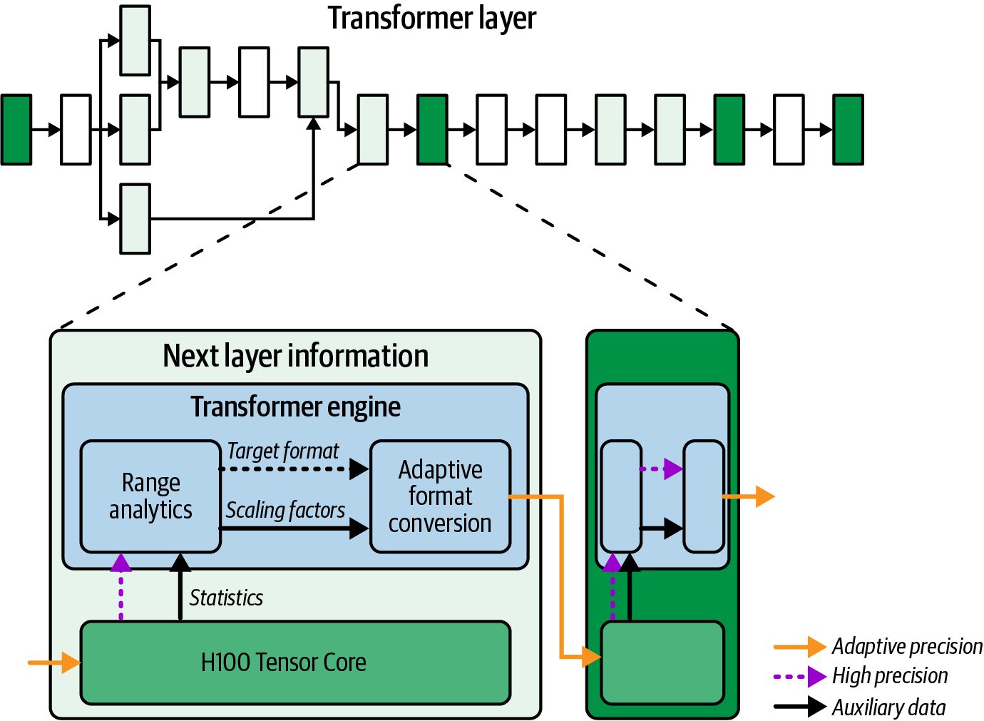
                     Use per-tensor or per-channel scaling depending on the kernel. It’s
                     recommended to explore per-tensor scaling for activations and
                     per-channel scaling for weights. For instance, when using FP8
                     E4M3 for KV cache quantization, it’s common to use per-tensor
                     scaling.
Per-block microscaling means that instead of using a single scaling factor for an entire tensor, it maintains a separate scale for each fixed-size block, typically 32 ele‐ ments, within the tensor. These separate scales adapt to local value distributions to preserve range and reduce quantization errors compared to single-scale quantization.
                     Always quantize with the calibration data that reflects your infer‐
                     ence workload. A one-time calibration on a subset of your training
                     data may not capture runtime usage patterns.
In practice, GPTQ (post-training quantization) and AWQ are commonly used for 4bit weights on LLMs—often with negligible accuracy loss. Open source tools from Hugging Face and others can apply these techniques automatically. The MoE expert structure makes weight quantization even more appealing since we can fit even more experts in memory using reduced-precision weights. As such, we can swap fewer experts to/from CPU memory. Additionally, we can use larger models with more active experts—and more expert replicas—if needed. Post-training quantization (PTQ) tools like GPTQ apply an approximate secondorder algorithm to quantize weights, layer-by-layer, down to 3–4 bits in a few GPU hours with almost no accuracy degradation. Newer GPTQ variants further refine this algorithm with asymmetric calibration and parallel computation. This reduces quan‐ tization error and extends efficient low-bit support to even larger models. AWQ identifies a small fraction of “salient” weight channels. Salient channels produce large activation magnitudes that have a disproportionately large effect on model output. AWQ preserves these channels using channel-specific scaling before casting all weights into 4-bit precision (e.g., INT4). NVIDIA’s TE knows how to use the channelspecific scaling factors on the preserved channels to maintain model fidelity.
                     Most AI frameworks like PyTorch and inference engines like vLLM
                     and TensorRT-LLM natively support loading GPTQ-quantized and
                     AWQ-quantized model checkpoints.
736 | Chapter 16: Profiling, Debugging, and Tuning Inference at Scale
Activation Quantization Quantizing activations along with weights can improve performance by using reduced precision for GEMM inputs—and potentially accumulators—using lowerprecision values. This will reduce memory traffic for both attention-based KV cache and intermediate activations in MLP layers. However, activation distributions can vary greatly with varying inputs. As such, acti‐ vation quantization can sometimes be challenging without proper fine-tuning or cali‐ bration. A middle ground is INT8 activation with calibration. This comes from NVIDIA’s INT8 mode, which uses per-tensor calibration and is used in TensorRT to choose scaling factors from activation histograms generated from a representative set of calibration data. SmoothQuant, a training/calibration-free PTQ method for 8-bit activation quantiza‐ tion, can be used to shift some of the quantization error from activations to weights using a simple row/column scaling algorithm. This lets us use INT8 for both weights and activations with minimal fine-tuning—leading to full INT8 inference with low (e.g., < 1%) accuracy loss.
               Using SmoothQuant activation quantization before applying
               GPTQ/AWQ on weights has been shown to preserve accuracy bet‐
               ter at low precision.
Post-Training Quantization Workflow The quantization techniques described previously are applied post-training—as opposed to quantization-aware training, which is done during model training (aka model pretraining). The typical workflow is to train or fine-tune the model in FP16/ FP32 and then run a post-training calibration script such as GPTQ or AWQ on a rep‐ resentative dataset to determine quantization parameters. Then you load the quan‐ tized model weights into the inference engine for serving. If needed, you can also run a small fine-tuning job to recover any lost accuracy; how‐ ever, this is typically not needed with the GPTQ and AWQ techniques. If you need full QAT, you can just run a few epochs of training with “fake quant” operations in the model graph to mimic low-precision math during evaluation. This will help you gauge expected accuracy at this precision.
Quantization Approaches for Real-Time Inference | 737
                     In practice, quantization-aware fine-tuning for LLMs is computa‐
                     tionally expensive and not always feasible. However, smaller cali‐
                     bration datasets of 1,000 prompts, for instance, can be used with
                     techniques like percentile clipping or LMS (loss-aware quantiza‐
                     tion) to fine-tune the quantization scales without full retraining.
It’s worth noting that you should be extra careful to balance the trade-off between compression and model robustness. Quantization can amplify certain errors. For instance, if a model was barely at the threshold of some factual knowledge, quantiza‐ tion might push it to make an error. Always validate on downstream tasks since PTQ makes assumptions that might miss subtle distribution shifts. As such, you should do extensive A/B testing of responses when using reduced-precision quantized models to make sure your evaluations show no regressions in quality or safety. If you see regressions, you should leave the model in higher precision—or try performing a light fine-tune in quantized form to restore performance.
Combining Weight and Activation Quantization Activation quantization to 4-bit remains challenging. Combining low-precision weight quantization with higher-precision activation quantization often produces the best trade-off between memory savings, compute efficiency, and accuracy. As such, many production systems use weight-only 4-bit (e.g., GPTQ/AWQ) quantization combined with 8-bit activation quantization. Specifically, in one W4A8 (8-bit activation) variant, the runtime unpacks INT4 weights, dequantizes to FP8 using learning or calibration scales, and executes the matrix multiply on FP8 Tensor Cores. This hybrid path is provided by inference engines like TensorRT-LLM and achieves near-lossless accuracy when properly cali‐ brated. This preserves the full dynamic range of activations while reducing weight storage by 4× compared to FP16. In contrast, the traditional INT4 and INT8 W4A8 scheme pairs 4-bit integer (INT4) weights with 8-bit integer (INT8) activations and runs the computations on INT8 Tensor Cores. This approach relies on histogram-based calibration to map activation ranges into INT8 without quality loss. Although the INT4/INT8 kernels can deliver slightly higher raw throughput with modern integer Tensor Core pipelines, they require careful activation calibration and don’t have as much dynamic range as FP8. A hybrid INT4 and FP8 approach combines the best of both worlds. In the hybrid approach, 4-bit integer (INT4) weights are unpacked and reinterpreted as FP8 inputs. The computation is then executed on FP8 Tensor Cores. This INT4 and FP8 hybrid
738 | Chapter 16: Profiling, Debugging, and Tuning Inference at Scale
W4A8 variant delivers near-lossless accuracy, massive memory-bandwidth reduc‐ tions, and excellent throughput on modern GPUs. For modern GPUs, two distinct low-precision paths are common in production. First, NVFP4 workflows use FP4 blocks with microscaling managed by the Trans‐ former Engine or TensorRT. Second, W4A8 workflows use INT4 weights with FP8 or INT8 activations executed using fused dequantization in TensorRT-LLM. Choose the path based on your model calibration and accuracy targets. In summary, quantization is one of the best ways to reduce inference cost. By cutting model size 2× or more, you effectively double the throughput per GPU. The tech‐ niques mentioned previously, including GPTQ, AWQ, and SmoothQuant, help you achieve these gains with minimal accuracy loss (e.g., often < 1% decrease).
               It’s recommended that you start with 8-bit weights and then evalu‐
               ate 4-bit weight-only quantization for additional gains. Then you
               can move to W4A8 only if you need maximum optimization and
               can spend time on calibration.
The next step is to eliminate any conversion overhead. By fusing quantize-dequantize operations directly into the compute kernels, you preserve the gains from using quantization.
Fusing Quantization-Dequantization Steps into the Execution Graph Modern inference engines use the TE to perform weight-packing and provide highefficiency mixed-precision math computations without the explicit calibration over‐ head of using INT8. These inference engines typically implement CUDA/Triton kernels to manually fuse “quant-dequant” steps into the execution graph when needed. These quant-dequant steps should be fused into the graph whenever separate Quan‐ tize/Dequantize kernels would introduce too many extra launches and negate the latency and bandwidth benefits of reduced-precision math. This is especially useful for inference backends that lack native fused INT8 support. Fusing quant-dequant into the main compute kernels is especially valuable for highthroughput inference pipelines to restore performance by removing bottlenecks caused by the conversion. Next, let’s explore various application-level optimizations supported by modern AI inference serving engines.
Quantization Approaches for Real-Time Inference | 739
Application-Level Optimizations Beyond the core model and system optimizations, there are several higher-level tech‐ niques that can significantly improve the performance and user experience of an LLM service. These methods operate at the application or inference-serving layer and improve how prompts are constructed and cached, how conversation history is pre‐ served, how requests are routed to different models, etc. These optimizations don’t involve modifying model weights or deploying new hard‐ ware. They are algorithmic and system-level improvements at the application layer. They can produce significant gains in efficiency and usability for “free” essentially, as they incur very little cost. In this section, we discuss a few such optimizations, including prompt compression, prefix caching and deduplication, fallback model routing, and streaming outputs. These strategies improve performance by reducing input size, avoiding redundant computations, providing graceful handling of different request types, and improving perceived latency for end users.
Prompt Compression Users often send very long prompts or conversation histories to an LLM. However, not all of this context may be necessary for producing an adequate response. Prompt compression refers to a set of techniques that shorten or simplify the input prompt without losing relevant information. Some system prompts or system-injected instructions are quite verbose (“You are ChatGPT, a friendly assistant designed to help users…”). Large system prompts will occupy a lot of space in the input context—and for every request. Prompt compression reduces the amount of work that the model needs to do. It directly translates to cost savings because a shorter input means fewer GPU computations.
                     Remember that the attention mechanism within a transformer-
                     based LLM model is O(n²) time complexity, where n is the size of
                     the input measured in number of tokens.
One simple form of prompt compression is removing redundant or irrelevant text. Consider a user prompt that contains a large chunk of text that is not relevant to answering their query. This can include a copy-pasted article in which the question relates to only one paragraph of the text. In this case, an upstream component could summarize or extract the relevant parts before feeding it to the LLM.
740 | Chapter 16: Profiling, Debugging, and Tuning Inference at Scale
Another form of prompt compression is dialogue summarization or truncation. For long chat histories, for instance, early parts of the conversation might no longer be relevant. The system can intelligently trim the conversation by summarizing older parts into a condensed form.
               Many production chatbots like ChatGPT do prompt compression
               automatically to stay within their context-length limits—and to
               speed up overall processing. This is a must-have for long-running
               conversations.
To do this, you can run a small LLM—or a traditional rule-based system—to summa‐ rize the oldest parts of the conversation into a brief summary. Often the policy is something like: when the conversation exceeds 75% of the maximum context length, summarize the oldest 25% of messages. This summary would then be prepended to the more recent parts of the conversation. And this becomes the new prompt going forward. When implementing prompt compression, make sure that no critical facts are lost. One approach is to have the model compress the prompt (e.g., generate a summary) and then verify the compressed prompt by asking the model questions about it. This way, your algorithm checks if key information was retained in the compressed ver‐ sion of the prompt. This prevents excessive latency on very long chats and keeps the model focused on the most recent parts of the conversation. By truncating earlier turns, you reduce the effective prompt length N, which reduces prefill self-attention work from N(N + 1) ÷ 2 (roughly O(N2)) to a smaller triangular cost for the shorter window. So while the cost approaches quadratic in the window size, the smaller N makes a significant dif‐ ference for very long conversations. A good summary can improve the response by filtering out irrelevant details. How‐ ever, a bad summary can omit important parts of the input that the user really cares about. Summarizing is best when the system is confident—or if the conversation is clearly digressing.
Prompt Cleansing Another technique is prompt cleansing. This is used to improve input formatting and tokenization. It helps reduce the amount of unnecessary whitespace or markup sent to the model. Tokenizers process every character, including spaces and newlines; the less unnecessary tokens we send, the better. While tokenizers like OpenAI’s tiktoken are very efficient with whitespace, large prompts with lots of markdown and HTML can bloat the token count. Simple
Application-Level Optimizations | 741
preprocessing like removing HTML tags and converting fancy quotes to plain text can avoid odd tokenizations and reduce the number of tokens. For instance, we can potentially reduce the amount of inference engine computations by not sending blank lines and repetitive punctuations that don’t impact the meaning of the input. This might save only a few tokens here and there, but it adds up across thousands of requests—especially for long input prompts. In some cases, we can compress prompts by using references instead of the full con‐ tent. For instance, if a user’s prompt includes a long piece of text that our system has seen before—perhaps because they are referring to a document that we have previ‐ ously stored—we could replace it with a reference like “file0”. The model could then be fine-tuned to retrieve the actual content for that reference— or we can handle it using a retrieval system. This crosses into retrieval-augmented generation (RAG) territory, which we won’t cover any further here, but the key point is that we don’t always need to feed the raw content through the model if there are alternative ways.
                     Some inference engines support setting a system prompt once per
                     session rather than sending it each time. This is a better solution
                     than recompressing the system prompt for each request.
We’ll discuss how to improve the efficiency of a large system prompt with prefix caching in the next section. But, for now, let’s use prompt compression to create a shorter and functionally equivalent set of instructions. For instance, the model can be trained to use special tokens or metadata to represent a long system prompt. This way, it doesn’t have to always process the long natural language version. Consider a 200-token system prompt full of text-based rules that can be replaced with 10 special tokens that trigger the same text-based rules expressed in 200 tokens of natural language. This requires that the model be trained to parse the metadata, derive the rules, and follow them. There’s ongoing research into “config” tokens that tell the model to load a certain pre‐ configured set of instructions for a given config token. Think of this like assigning a unique ID for a given prompt prefix (e.g., system prompt). It’s common to fine-tune a model to recognize tokens like <POLICY_A> as a stand-in replacement for a long, 500word policy, for example.
742 | Chapter 16: Profiling, Debugging, and Tuning Inference at Scale
               The Hugging Face Transformers library implements the popular
               CTRL approach. This is a good place to start working with config
               tokens for prompt trimming.
Using special tokens and metadata to replace long system prompts is more of a train‐ ing consideration. But it can provide a massive inference speedup if it reduces the size of the prompt and decreases prefill overhead. At scale, this directly translates to less compute needed per query—and more cost savings.
Prefix Caching Often multiple requests to an LLM share a common prefix in their input, as many queries might start with the same system prompt. Instead of recomputing the model’s output for the same prefix each time, you can compute it once and reuse the same KV cache for subsequent requests. This technique is known as prefix caching, sometimes called prefix memoization. With prefix caching, the transformer’s state, including the keys and values in the attention layers, is stored and reused when a request with the same prefix appears again.
               Prefix caching can turn what would normally be O(N × L) total
               work (N requests of length L) into O(N + L) work by reusing the
               cached prefix computations for repeated parts.
vLLM implements prefix caching (enable_prefix_caching=True) to avoid recompu‐ tation. It first identifies if an incoming prompt’s first N number of tokens match a prefix that’s already in the cache from a previous request—or earlier in the same ses‐ sion. If so, vLLM avoids an expensive attention recomputation for those N tokens— and just copies data from the cached KV into the new context. Make sure you have prefix caching enabled—and with a sufficient memory allocation. An inference engine like vLLM can automatically group incoming queries into microbatches to achieve high GPU utilization, amortize overheads across many requests, and keep latency low using continuous batching, for instance. Make sure that if you’re not using an inference engine like vLLM directly, you look for ways to use prefix-sharing in your stack. Prefix caching can speed up workloads with repeated prefixes. Consider a scenario in which we want to ask 10 separate questions from a long document. Each would include the document in the prompt followed by one question, such as, “[Long docu‐ ment text] Question 1: …”, “[Long document text] Question 2: …”, etc.
Application-Level Optimizations | 743
The document text is the same across all 10 prompts. Normally, the model would need to reprocess the KV entries for the whole document for each question. This would lead to 10× redundant work as the model will re-encode the long document 10 times. With prefix caching, it encodes it once, and each subsequent question incurs the compute only for the smaller question suffix. Specifically, with prefix caching, the first query would compute the transformer states for the document portion, and for subsequent queries, the model can jump straight to processing the “Question 1: …”, “Question 2: …” parts since the document’s content matches a prefix found in the KV cache. With prefix caching, your inference engine can produce near-linear speedups. For instance, if you ask 10 separate questions on one document, these will be processed roughly 10× faster with prefix caching than without because the long document’s attention is calculated only once instead of 10 separate times. Another application of prefix caching is chat sessions since the conversation history is a common prefix for each new “turn” in a “multiturn” chat session. When the end user sends a new message, the earlier messages form a prefix that keeps growing. Optimized inference systems keep the KV cache from the last turn and compute KV only for the new user message. This is what most chat models like ChatGPT are doing if you don’t reset the conversation in between turns.
                     The benefits of prefix caching are most noticeable in interactive
                     settings—especially if users follow up quickly in the same context/
                     session. In this case, the second answer will come much faster than
                     the first since the prefix (conversation history) is already cached.
In addition to supporting state in their ChatGPT consumer product, OpenAI sup‐ ports stateful conversations in their API as well, which uses a form of prefix caching—among many other optimizations—behind the scenes. For stateless API invocations, prefix caching can achieve a similar effect if the client passes the conver‐ sation history. In this case, the server can retrieve the precomputed hidden state from the prefix cache—up to the last turn. It will then continue from there with the new user message. To implement this yourself, you can hash the conversation histories. This will give you a consistent key to look up in the cache. However, you will have to manage mem‐ ory carefully, as storing entire KV caches for many conversations can use GPU mem‐ ory very quickly. vLLM’s paging helps by paging inactive caches to CPU memory—or disk—and paging them back into GPU memory on a cache hit.
744 | Chapter 16: Profiling, Debugging, and Tuning Inference at Scale
You can also deduplicate portions of a prompt across multiple requests—or even within a single request. Here, deduplication refers to combining identical subprompts to compute their transformer states just once. For instance, if two users send the exact same prompt prefix at nearly the same time, the system could merge the two prompts and process them only once. This can also happen within a single request if the input has repeated sequences. This is more common in training, which uses techniques like memoized decoding to deduplicate repetitive text. In inference, it’s rare to get long, repeated input sequences in the same request, but it is possible.
                If your workload has many repeat queries on the same prefixes, you
                should allocate more memory to the cache to maximize hits. Con‐
                versely, if prefixes are rarely reused, you should use a smaller cache
                —or even disable prefix caching entirely. Always measure prefix hit
                rates in production and tune accordingly.
The prefix cache is typically implemented as a token-sequence trie (pronounced “try”). A trie, often called a prefix tree, is a tree-based data structure in which each edge represents a single token and each node encodes the sequence of tokens from the root to that point. In a token-sequence trie, every observed prompt prefix is stored as its own path of tokens. This enables fast lookups of shared prefixes. When a new request arrives, the inference engine traverses the trie—token by token—from the root until it can no longer match the next token. The sequence of matching tokens lands at the node that completes the longest-cached prefix, as shown in Figure 16-8 for an example system prompt, “You are ChatGPT, a friendly assistant designed to help users…”
Figure 16-8. Prefix cache implemented as a trie data structure
Application-Level Optimizations | 745
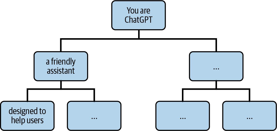
At this point, the system reuses the shared KV cache data (clones the pointers) and resumes decoding but only for the remaining tokens in the sequence. This avoids redundant self-attention computations for the already-cached prefix since the atten‐ tion scores for this prefix have already been computed. SGLang’s RadixAttention uses a compressed trie, or radix tree, over entire token sequences. This type of prefix cache collapses token sequences into single edges in the tree to save space. Each node in the tree points to a KV‐cache tensor stored as a con‐ tiguous GPU page that holds the prefix’s KV cache. The RadixTree data structure is space efficient and provides rapid prefix searches, efficient insertions, and LRU-style eviction. Here is pseudocode that shows a KV cache lookup using a radix tree during token generation: # Simplified RadixAttention KV cache example # radix_attention_example.py
radix: RadixTree = RadixTree() # holds edge labels + node.cache pointers
      def generate_with_radix(prompt_tokens: List[int]):
          # 1) Find longest cached prefix
          node, prefix_len = radix.longest_prefix(prompt_tokens)
          # shallow-clone the KV cache for that prefix
          model_state = ModelState.from_cache(node.cache) # refcount bump
           # 2) Process remaining prompt suffix
           for token in prompt_tokens[prefix_len:]:
               model_state = model.forward(token, state=model_state)
           # 3) As we go, insert or split edges in the radix tree
               matched = prompt_tokens[:prefix_len + 1]
               # insert returns the node for this full prefix
               node = radix.insert(matched, cache=model_state.kv_cache)
prefix_len += 1
           # 4) Now generate new tokens autoregressively
           output_tokens = []
           while not model_state.is_finished():
               token, model_state = model.generate_next(model_state)
               output_tokens.append(token)
                # cache each generated prefix as well
                matched = prompt_tokens + output_tokens
                node = radix.insert(matched, cache=model_state.kv_cache)
return output_tokens
746 | Chapter 16: Profiling, Debugging, and Tuning Inference at Scale
When generation begins, the engine calls radix.longest_prefix(prompt_tokens) to walk multitoken edges down the radix tree until it reaches the deepest node matching the prompt’s longest cached prefix. It then does a lightweight clone of that node’s KV cache page using ModelState.from_cache(node.cache). This seeds model_state without recomputing any self-attention for the cached prefix. Next, it processes only the unseen suffix of the prompt—token by token—and updates the radix tree on the fly. For each new token, it calls radix.insert(...), splits edges, or creates new ones as needed. It then stores the intermediate model_state.kv_cache at each new node. Once the entire prompt has been consumed, the loop switches to the autoregressive decoding phase, which generates new tokens with model.gener ate_next(model_state). Similarly, this inserts each generated prefix into the radix tree. This approach minimizes redundant computations, uses space-efficient storage of KV pages, and performs fast prefix lookups—all while supporting incremental cache updates. SGLang’s KV cache design automatically captures all common reuse patterns, includ‐ ing multiturn chats, few-shot examples, and branching logic. At the same time, it makes sure that shared prefixes are fetched as large, coalesced memory chunks for efficient GPU access. Knowing when to invalidate the cache is always a challenge. If the cache memory is needed for other things, you may need to evict some prefixes. Caching systems sup‐ port different policies, such as “least recently used” (LRU), in which the least recently used prefix gets evicted first. SGLang’s RadixAttention, for instance, will lazily evict the least recently used radix-tree leaf when GPU memory is scarce, as shown in Figure 16-9. This is a prefix cache tree structure—and LRU eviction policy—used by SGLang for multiple incoming requests. This example is based on an awesome SGLang blog post from LMSys.
Application-Level Optimizations | 747
Figure 16-9. Prefix cache evolution for multiple requests (source: https://oreil.ly/7LBoC)
748 | Chapter 16: Profiling, Debugging, and Tuning Inference at Scale
Here, there are two chat sessions and multiple queries across those chat sessions. The label of each is a sequence of tokens (e.g., substring). Green nodes represent new nodes in the tree. Blue nodes are cached nodes that are currently being accessed. Red nodes have been evicted. Here is the breakdown of each step:
 1. The initial empty radix tree is empty.
 2. The server processes the incoming prompt “Hello!” and responds with the LLM-
    generated “Hi!” With this simple response, many tokens are added to the tree as a
    single edge. This edge is linked to a new node in green. Specifically, the system
    prompt, “You are a helpful assistant”; the user message, “Hello!”; and the LLM
    response, “Hi!” are consolidated.
 3. The server receives a new prompt. This is the first turn of the multiturn conver‐
    sation. The server successfully looks up the prompt prefix in the tree and reuses
    its KV cache data. A new turn is added to the tree as a new green node.
 4. A new chat session begins, and node b from step 3 is split into two separate
    nodes. This lets the two chat sessions share the system prompt.
 5. The second chat session from step 4 continues. Memory is limited, however, so
    node c from step 4 must be evicted, and it’s shown in red. A new turn is
    appended after node d in step 4.
 6. The server receives a new prompt (query). After processing, the server inserts the
    prompt into the tree. This requires the root node to split because this new
    prompt does not share any prefix with existing prompts/nodes.
 7. The server receives a batch with more prompts (queries). These prompts share
    prefixes with the prompt from step 6. As such, the system splits node e from step
    6 and shares the prefix.
 8. The server receives a new message from the conversation in step 3 (the first chat
    session). In this case, it evicts all nodes from the second chat session in step 5
    (e.g., nodes g and h). This is because they are the least recently used (LRU) at that
    moment.
 9. The server receives a message requesting more answers for the query in node j
    from step 8. Due to memory limitations, the system is required to evict nodes i,
    k, and l from step 8.
This example demonstrates how prefixes are shared between multiple requests. In addition, it shows how an LRU cache-eviction policy works in the context of prefix caching. Next, let’s turn to using a cascading model deployment pattern to better uti‐ lize GPU resources.
Application-Level Optimizations | 749
Model Cascading and Tiered Model Deployment Not all queries require the power (and cost) of the largest, state-of-the-art models. Some user requests are simple enough to be answered by a much smaller, faster, and cheaper model. Choosing the right model is called model cascading or fallback model routing. To implement model cascading, you can use tiered model deployment. This is an approach that maintains multiple models of different sizes and abilities. For each incoming request, we dynamically choose which model to use based on query com‐ plexity, required precision, or current system load. Consider a question-answer (QA) inference deployment with both a large 700billion-parameter state-of-the-art model and a smaller 70-billion-parameter model that is faster and cheaper to host since it requires fewer GPU resources. If a user asks a very straightforward and factual question (as determined by a classifier or heuris‐ tic), the 70-billion-parameter model might handle it well. For straightforward questions, you can route the query to the smaller model, which will respond in 50 ms instead of 500 ms with the 700-billion-parameter model. If the small model’s answer is deemed unsatisfactory due to low confidence (determined by the logits returned in the response), the system can route the question to the bigger model. This two-stage approach can reduce overall average latency and compute usage— although individual requests may experience longer latencies if they’re routed to both models due to lack of confidence in the small model’s initial response. It’s widely believed that many commercial AI services, such as ChatGPT, use this approach of routing simpler queries to smaller, faster models to reduce cost and latency. In practice, routing, say, 60% of queries to a 10× smaller model can cut your inference compute costs significantly—potentially a 5× overall cost reduction if designed and tuned properly. This is because the expensive model is used only when needed.
                    Maintaining multiple models and a routing system is an engineer‐
                    ing overhead, as you need to monitor not just one model’s perfor‐
                    mance but also the second model, the interplay between the two
                    models, and the routing system. Pursue this only if your traffic vol‐
                    ume and cost structure make it worthwhile.
Implementing model cascading requires a query classifier or heuristic mechanism to assist the model-routing decision. And this is a relatively difficult problem to solve correctly, as the mechanism often requires continuous adaptation, comprehensive heuristics, and constant router tuning. As such, many organizations still rely on heu‐ ristic and rule-based routers using offline analysis to update the decision criteria.
750 | Chapter 16: Profiling, Debugging, and Tuning Inference at Scale
One approach is to consider this a speculative problem, similar to speculative decod‐ ing described earlier. You can first run the smaller model in a draft mode and have it generate the answer with its confidence score. If confidence is high, just return the response. If not, call the bigger model. Make sure that if the big model is needed, the additional latency of the small model doesn’t make the user wait too long. In practice, you might run the small and large models in parallel when you suspect that the question is hard. This overlaps the small model’s latency with the large model. This seems wasteful and counterintuitive, but it can be beneficial for some latency-sensitive use cases to keep latency low—at the expense of additional compute. Another approach is to train a separate classifier for well-known user queries ahead of time. For instance, you can classify complexity and ask, “Does this question require the big model’s extensive knowledge or reasoning?” If not, use the small model. It’s important to note that this classifier will itself need periodic retraining as user queries evolve over time. Also, it introduces another component that can degrade and fail—and therefore needs to be monitored. Make sure this model is lightweight, fast, and robust—otherwise it becomes a new bottleneck in your inference system. It’s common to use a simple heuristic initially. For instance, if the user’s query is short and factual, such as “What’s the weather today?” or “Who is president of X?”, you can just use the smaller model. For longer prompts (e.g., > 50 tokens) or more creative queries that contain words like explain, analyze, or elaborate, you can just send it to the big LLM directly and bypass the smaller model. You should log and tag every request with which model handled it (e.g., “small” ver‐ sus “large”)—and whether it fell back. This lets you break down latency, accuracy, and fallback counts by model. This tagging data also lets you monitor the dispatchers’ decisions. By counting the number of times when the small model’s answer was rejected, you can identify pat‐ terns that may lead to retraining the smaller model or improving the routers’ heuristics. Conversely, if the small model handles many queries well, you can use this informa‐ tion to raise its confidence threshold. This will increase the small model’s usage, reduce response latency, and improve the end user experience. You can also route based on capacity. If the big model cluster is at maximum load, rather than queue requests and increase latency, we might temporarily route less criti‐ cal requests to a smaller model, which might not be as good but still gives some answer quickly. This is a form of graceful degradation under heavy load. The user might notice a quality dip, but it’s better than timing out or waiting excessively.
Application-Level Optimizations | 751
Many AI services do this intentionally. For example, during peak loads, free-tier users might silently get routed to a smaller model to free up the larger model for premiumtier (paid) users. This is a realistic trade-off when resources are constrained.
                     We will cover more advanced dynamic and adaptive inference
                     server capabilities in Chapters 17–19. These features depend heav‐
                     ily on the current system load, including available GPU memory,
                     memory bandwidth utilization, KV cache utilization, etc.
Another form of model cascading is based on the content itself. For instance, if a user asks something that the LLM refuses to answer due to safety, some inference systems will fall back to a special model fine-tuned specifically to handle unsafe prompts—or even to a retrieval system. This is more about content policy than performance, but it’s still an important con‐ sideration for your model-routing logic. And often the fallback model is much smaller, so this actually ends up being a performance win since it handles the unsafe request quickly—and frees up the main model to handle the safe queries. From a deployment perspective, multimodel setups require careful scaling since each model needs enough instances to handle its portion of traffic. Sometimes one model might become a bottleneck if many simple queries come in, for instance, and the small LLM is saturated while the big model sits idle. You can autoscale and run more or fewer instances of the small model during certain times of day—or even dynamically shift GPUs from the large model pool to the small model pool as needed using container orchestration.
Streaming Responses To improve the “perceived” performance of your inference system, you should stream the output tokens as they are generated. This is much better than forcing an end user to wait for the full completion to finish before they see a response. This way, users can begin reading and processing information as it arrives. This can make the effective interaction much faster—even if total time is the same. Humans can read anywhere from 200 to 300 words per minute, which translates to approximately 4–7 tokens per second—or up to 13 tokens per second for faster read‐ ers. Maintaining this pace of streaming response is ideal. Given that every perfor‐ mance decision comes down to trade-offs, this is an important metric to consider when making optimization choices, planning capacity, etc.
752 | Chapter 16: Profiling, Debugging, and Tuning Inference at Scale
                It’s important to monitor your system’s token throughput against
                this human reading rate. For instance, if you find your system is
                streaming at only 2 tokens/sec due to model latency, that’s a sign to
                optimize further.
Streaming is supported by most modern inference engines, including vLLM, SGLang, and NVIDIA Dynamo. When you enable streaming, the server flushes tokens to the client using WebSockets, Server-Sent Events (SSEs), the HTTP Streaming protocol, etc. And it should do this immediately when the tokens are generated to meet the 4– 13 tokens-per-second human-reading metric mentioned earlier. The model effectively generates one token at a time—except when using speculative or multitoken decoding techniques like EAGLE or Medusa, respectively. As such, the system needs to group those generated tokens into batches of 2–5 tokens, flush the stream, and send the batched tokens back to the end user. It’s important not to accumulate too many tokens in a batch before flushing, or you defeat the purpose of streaming. On the other hand, sending one token per packet may be inefficient due to overhead. Often frameworks flush on every newline or endof-sentence token. For example, if an answer is 100 tokens and takes 5 seconds to fully generate, with streaming, the first batch of tokens would arrive after 0.25 seconds if the batches are 5 tokens each (5 tokens ÷ 20 tokens per second = 0.25 seconds). This would be fol‐ lowed by a steady stream of token batches until the response is complete. This way, the user can start reading after just 0.25 seconds. Without streaming, the user would stare at a blank screen for 5 seconds, then sud‐ denly see the whole answer shown all at once, which is not ideal. This could lead to rage clicking and other forms of user frustration. From a performance standpoint, streaming imposes a slight overhead due to addi‐ tional, small network packets being sent instead of one big message. But this over‐ head is usually negligible compared to the model’s computation time—and compared to the improved end-user experience. Using HTTP/2 and persistent connections helps reduce overhead by sending tokens as a continuous stream without needing to reestablish connections.
Application-Level Optimizations | 753
                     Be mindful of Nagle’s algorithm and delayed acknowledgments.
                     The interaction can add tens of milliseconds of delay and, on some
                     stacks, up to roughly 200 ms in worst-case settings. Use TCP_NODE
                     LAY and, where available, quick-ack or reduced delayed-ack timers
                     to minimize token flush latency. These help reduce token‐send
                     latency, which is critical for real‐time streaming. The downside is
                     more small packets fill the pipe—and bandwidth efficiency is
                     reduced. But keep this in mind when tuning for ultralow latency.
It’s important to properly manage flow control such that if the client is slow to con‐ sume the stream due to network issues, for instance, you don’t want to block the model’s generation. Ideally, the inference engine will continue generating the whole response—even if the client falls behind consuming the stream. The system should use separate threads and CUDA streams to send the data back to the end user. This way, the main token generation loop isn’t interrupted by issues while sending the response. The inference engine maintains a bounded buffer to manage flow control and prevent unbounded memory growth. This can happen if a client stalls or disconnects. It’s important to handle these types of edge case scenarios as they are fairly common in production scenarios. In practice, you might allow up to 50–100 tokens to accumulate. Beyond a certain limit, the inference engine can either pause generation or close the connection completely. This way, if a client drops mid-generation—or simply can’t keep up due to a slow connection—the engine can stop producing tokens and free those resources to handle other requests. Choosing the buffer limit involves balancing memory use and user experience. This is rarely an issue for short responses, but it is somewhat common for very large responses—especially for slower consumer connections. Another trick to improve flow control is to use token pooling. If the model generates tokens faster than needed for streaming, the system can intentionally add a delay to smooth out the rate of generation. For instance, if the model bursts out 20 tokens in 0.5 seconds because it was a simple part of the response, for instance, sending them all at once can display a big chunk and then pause for the next part. You may prefer your application’s UI to use a steadier typewriter effect. In this case, you can introduce an artificial stream delay like 50 ms between token sends. This doesn’t affect actual latency much, and it improves the UX by avoiding janky bursts of tokens. You can make the token-pooling delay configurable to adapt to different UXs for dif‐ ferent types of users (e.g., paid users, free users, etc.). Paid users can stream faster,
754 | Chapter 16: Profiling, Debugging, and Tuning Inference at Scale
while free users will be throttled a bit. This can help manage load with limited resources. Streaming responses also allow end users to start evaluating the intermediate results and take action before the response completes. For instance, if the user sees the first part of the answer and realizes it’s not going in the direction they want, they can stop the generation using a Stop or Interrupt button. This saves unnecessary compute and improves the UX as the end user doesn’t have to wait for a bad completion to finish before they provide their feedback. You should monitor—or at least measure—early stops. Too many explicit stops might indicate an issue with the model’s relevance. If you see many users stopping at a certain point, it might indicate the model often goes offtrack or is too verbose beyond that length. This could inform you that the model needs additional fine-tuning to make it more concise. Or you can make adjustments to the maximum tokens generated and sent to the end user. Or the early stops could be caused by a frustrated “rage click” type of user who changes their mind frequently. Either way, it’s best to allow the user to interrupt the token-generation process. This lets the inference cluster reclaim the resources to han‐ dle other requests. In short, streaming is a must-have for a responsive LLM service. It doesn’t increase raw throughput—if anything, it adds a slight overhead, but it improves the userperceived speed of the system. Streaming responses should be implemented carefully to not interfere with generation. Different threads and CUDA streams should handle sending responses back to the end user so that the main token generation loop isn’t stalled on flakey end-user network connections.
               It’s recommended that you continuously profile your end-to-end
               latency with streaming enabled versus disabled in a test environ‐
               ment. Make sure that token emission is evenly spaced—and that no
               significant bottlenecks like lock contention or I/O waits are intro‐
               duced. Tools like Locust are Python friendly and can simulate cli‐
               ents. This lets you test your low-latency streaming workloads at
               scale.
Debouncing and Request Coalescing Many production systems also implement UX features called debouncing and request coalescing. By debouncing, or pausing, before responding, the system can recognize if a user sends multiple requests in quick succession—either by accident or from rage clicking, as shown in Figure 16-10.
Application-Level Optimizations | 755
Figure 16-10. Debouncing pauses a bit before performing an action
In this case, the system can either coalesce the multiple queries into one query or drop all but the latest query. These types of application-level guardrails help reduce excessive, repeated, wasteful load on the backend. For example, if a user double-clicks Submit or sends two very similar queries within a second, the system can drop the duplicate. Rage clickers impatiently resubmit multi‐ ple times when they are frustrated—often because of the application’s poor response time. Ironically, debouncing and request coalescing can create more latency, frustrate the “rage” user segment even more, and cause them to click even more! In this case, it’s helpful if the UI disables the input while a request is in flight. This can prevent double-clicking at the UI level. But it’s also good to have server-side protection in place, as well.
                     Modern inference load balancers support a debouncing interval.
                     Use a modest interval (e.g., 2–5 ms), and find a good trade-off
                     between batching efficiency and added latency. And next time you
                     submit something in ChatGPT, notice the debouncing delay. It’s a
                     bit annoying now that you know about it, isn’t it?!
Token Output Limits and Timeouts Because response token counts directly influence latency, you can implement output length limits or timeouts. This kind of application-layer constraint can prevent run‐ away generations in which the model keeps generating beyond a reasonable number of tokens. Token output limits and timeouts help maintain consistent latencies. They also pre‐ vent malicious and accidental prompts from causing extremely long generations that
756 | Chapter 16: Profiling, Debugging, and Tuning Inference at Scale
could tie up GPU resources. Many public APIs set strict output limits for exactly this reason. It’s both an abuse prevention mechanism as well as a performance safeguard. Always set server-side timeouts, as well. For example, if a generation exceeds 30 sec‐ onds, return a partial result or an apology. Users expect quick failures rather than a hanging response.
               Also monitor if your model tends to ramble. Applying a moderate
               token limit, perhaps 4,096 tokens for a chat answer, can actually
               improve quality by keeping the model on track and avoiding long
               answers.
It’s important to choose these limits and timeouts based on user needs. These limits keep latency predictable and also cap the worst-case compute scenario. This helps with capacity planning, etc. In summary, the combination of input optimizations (e.g., compression and cleans‐ ing), caching, smart routing, and UX optimizations (e.g., streaming data) can reduce the workload, reduce the size of the inference cluster, save cost, and improve user sat‐ isfaction. These application-level strategies complement the low-level optimizations from earlier sections—rounding out the holistic approach to improving LLM serving performance.
Key Takeaways The techniques in this chapter show that efficient LLM serving is a holistic engineer‐ ing effort that combines modern GPU hardware, novel software optimizations, and comprehensive monitoring. Profiling tools identify the bottlenecks. Systematic debugging techniques fix the issues. Here are some key takeaways from this chapter: Comprehensive profiling Perform end-to-end profiling across the inference stack. By measuring latency and resource usage at each stage using profilers, engineers can pinpoint slow‐ downs and inefficiencies. This data-driven approach guides targeted optimiza‐ tions to eliminate bottlenecks. Monitoring and observability Implement robust monitoring for deployed inference services. Track key metrics such as latency percentiles, throughput, GPU utilization, and memory usage in real time to detect regressions or resource saturation early. Use logging and trac‐ ing to get visibility into per-request processing and identify hotspots or anoma‐ lies in a large-scale workload.
Key Takeaways | 757
Debugging and iterative tuning
   By adopting a systematic debugging workflow, you can resolve performance and
   correctness issues quickly—even across tens of thousands of nodes. This way,
   when an unexpected spike occurs (e.g., decrease in throughput or increase in
   latency), you can easily drill down from the high-level symptom to the low-level
   issue.
Validating optimizations with metrics
    Tools such as GPU debuggers, memory leak detectors, and performance-related
    unit tests help verify that optimizations like quantization and kernel fusion do
    not introduce silent performance and correctness errors. This iterative tune-and-
    test cycle is essential for maintaining high performance and reliability with each
    new optimization released into production.
Efficiency and cost optimization
     Focus on improvements that make inference more cost-effective. Every optimiza‐
     tion that increases throughput and utilization will directly improve the cost-per-
     query. By profiling and refining the system, teams can serve more requests with
     fewer GPUs. This leads to significant savings in infrastructure costs and power
     efficiency.
Conclusion Profiling, debugging, and full-stack system tuning are critical for maintaining effi‐ cient, reliable, and cost-effective LLM inference at scale. As model sizes grow toward multi-trillion parameters, production clusters are scaling toward hundreds of thou‐ sands and even millions of GPUs per deployment. Continued codesign of software and hardware remains essential at this scale. It’s no longer enough to rely on just hardware to increase performance—especially as power is becoming a limiting factor. Both the software and hardware need to be codesigned and continuously tuned together—and at every layer in the stack. An optimized inference infrastructure provides fast response times for end users, predictable and stable system behavior, and low operational costs. Only then can you deliver inference systems that serve the largest and most powerful models in the world. In the next chapters, we will dive deep to understand and optimize the most com‐ pute, memory, and network intensive parts of modern LLM inference systems: calcu‐ lating (prefilling) the KV cache, sharing it with all workers in cluster, and using it to generate (decode) new tokens.